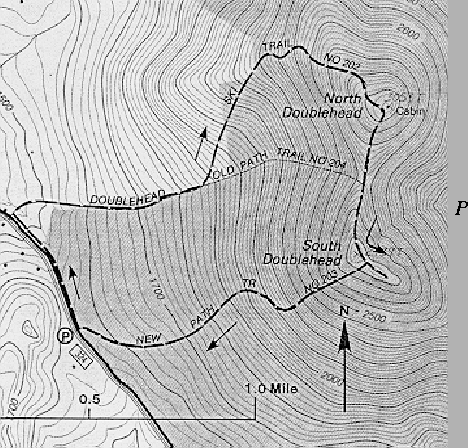
A contour plot for f is a plot of a portion of the domain of f showing several level sets of f for different values c.
startsection section10mm-.5 Discussion 14 Contour Plots
In this discussion, we will investigate a single contour plot in order to determine what we can learn about a function from its contour plot. First, we must define what we mean by a contour plot.
The contour curve or level set of a functionUsually the collection of values c that correspond to the level sets in a contour plot are evenly spaced values, for example, 5, 10, 15, 20, and so on. The values c for the level curves are indicated on the plot.for the value c, is the subset of
, given by

A contour plot for f is a plot of a portion of the domain of f showing several level sets of f for different values c.
startsection subsection10mm.5 Exercises These exercises refer to the accompanying contour plot of Doublehead Mountain in New Hampshire. In this case, the function f under consideration is altitude above sea level measured in feet. Of course, there is no symbolic form for such a function. Note that the contours on the plot are for values c that are separated by 20 feet.
 |
startsection section10mm-.5 Discussion 15 Plotting Functions of Two Variables in Maple
This is a LATEXversion of a Maple worksheet. The worksheet is available in the directory
/home/stu/courses/math141.
startsection subsection10mm.5 Introduction
This discussion will introduce the Maple commands for plotting functions of two variables that we will be using in this course. These commands will allow us to plot complicated functions with ease. However, we want to emphasize that it is not sufficient just to be able to plot functions, we must also be able to interpret the plots.
The first part of this discussion introduces the commands and the second part of the discussion asks you to use these commands to analyze several functions of two variables.
startsection subsection10mm.5 Plotting Commands for Functions of Two Variables
As we have seen previously, the plotting commands that we will be using are contained in the Maple package ``plots''. In order to use the commands in this package, you must load it at the beginning of your Maple session using the ``with'' command. This command is given below. Enter this command before continuing.
with(plots):
We will use plot commands, contourplot, plot3d,
and contourplot3d . (Words in green are hyperlinks to the
corresponding help pages.) The first two display 2-dimensional plots
of the domain of the function. The second two display 3-dimensional
plots of the graph of the function. The syntax of each of the plot
commands is similar. To use each of these commands we will first
define the function we wish to plot in Maple. We do this using the
:= construction, for example, the function
f(x,y) = x2-y2is defined using the command:
f:=(x,y)-> x^2-y^2;After defining the function, we can use the plot commands below to generate the different graphical representations of f.