Parametric Curves and Vector Fields

startsection section10mm-.5 Discussion 6 Parametric Curves

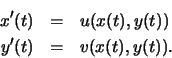
 In one variable calculus we considered mathematical models for rectilinear motion, that is, motion in a straight line. We modelled the position of an object with a function of time, $s : [a,b] \rightarrow {\bf R}$. For any time t, $a \leq t \leq b$, s(t)represented the position of the particle on the s axis at time t. Here we want to build on that model to consider the motion of an object in the plane or in space.

startsection subsection10mm.5 Exercises

1.

Let us begin with an object moving in a plane so that as time evolves, the object traces a curve in the plane. How would you use functions to describe the motion of the object? Explain how you can use your description to determine the position of the object at each instant of time.

2.

Let us put your method of description into practice. A bridge 600 feet long spans a canyon that is 1500 feet deep. For no particular reason you carry a stone as you walk from one end of the bridge to the middle of the bridge (at a speed of $6\mbox{ ft/sec}$), you look over the railing for 5 minutes, then drop the stone into the canyon.

(a)

Use your method of describing the motion of an object to give a mathematical description of the motion of the stone from the time when you begin walking across the bridge until the stone hits the river at the bottom of the canyon.

(b)

Assume now that instead of dropping the stone, you throw it straight down at 20 ft/sec. Will the same mathematical description suffice to describe the motion of the stone this time? Explain why or why not, and if not, provide a correct mathematical description.

3.

How would you extend your description of the motion of an object in the plane to the motion of an object in space? Does your description specify the position of the object in space at each instant of time?

startsection section10mm-.5 Discussion 7 Plotting Parametric Curves Using Maple

 

This is a L^ATEXversion of a Maple worksheet. The worksheet is available in the directory /home/stu/courses/math141.

startsection subsection10mm.5 Introduction

In this discussion, we will use Maple to visualize and investigate parametric curves. (See Section 2.1 of the text.) Maple can be used plot the image of a parametrization $\boldsymbol{\alpha}(t) = (x(t),y(t))$ in the plane, or $\boldsymbol{\alpha}(t) = (x(t),y(t),z(t))$ in space, on a domain [a,b].

As you work through this discussion, you might find it valuable to use the built-in Maple Help utility, which can be accessed by selecting Help from the Menu bar at the top of this window. In addition, you might want to have available the document ``Maple for Vector Calculus: A Summary of Useful Commands,'' which appears at the beginning of the collaborative learning workbook. (For an on-line overview of Maple plot commands see the worksheet maple_intro.mws)

The plotting commands we will be using are contained in the Maple package ``plots'' In order to use the commands in this package, you must load it at the beginning of your Maple session using the command

   with(plots);

To execute this command, move the cursor to the end of the input line and hit ``enter''.

Maple responded with a list of all the commands that are contained in the package ``plots.'' Notice that input statement ended with a semi-colon. All Maple input must end with a semi-colon or a colon. A colon suppresses the output. If we do not want to see the list of commands contained in the package ``plots'', the above ''with'' statement should be followed by a colon rather than a semi-colon.

startsection subsection10mm.5 The Maple Plotting Commands The basic two-dimensional plotting command plot for graphing functions y=f(x) can also be used to plot the image of a parametrization in the plane. To plot the image of the parametrization given by two expressions in t on the interval [t₀,t₁], first we will define the function $\boldsymbol{\alpha}$ using the := construction. Thus we will define $\boldsymbol{\alpha}(t)$ in Maple by

    alpha:= t->(expression1,expression2);

then we can use

    plot([alpha(t),t=a..b]);

to plot the image of $\boldsymbol{\alpha}$ in the interval [a,b]. To plot several curves at one time, we will define the functions Maple and then enclose a list of bracketed expressions in braces within the plot command.

    plot({[alpha(t)1,t=a..b],[alpha2(t),t-a..b], ...});

Note that each curve is plotted in a different color.

To plot a parametric curve in space we must use the Maple command spacecurve from the package plots. The syntax for this command is similar to that for the parametric form of the plot command that was explained above. For example, the image of parametrization given by three expressions in t on the interval [a,b], can be plotted using

    alpha:=t->(expression1,expression2, expression2);
    spacecurve([alpha(t),t=a..b]);

For further information about plot and spacecurve consult the Maple Help utility.

startsection subsection10mm.5 An Example

In this example we will first use Maple to plot a circle centered at the origin. The function $\boldsymbol{\alpha}(t) = (R \cos(t), R \sin(t))$ parametrizes motion about a circle of radius R centered at the origin. To define this function in Maple, enter the following commands:

 R:=2;
 alpha:= t-> R*cos(t), R*sin(t);

Since we set R = 2, the image of alpha is a circle of radius 2centered at the origin. To plot this image on the interval $[0, 2\pi]$, enter the following command.

 plot([alpha(t),t=0..2*Pi]);

You can plot circles of different radii by changing the value of R on the command line above and then reentering the command which defines alpha and the plot command.

We can also use the display command to plot several different images on the same set of axes. For example suppose we want to plot alpha from above along with the image of the parametrization beta given defined on the next line.

 beta:=t->1+2*cos(t), -1+2*sin(t);

In order to plot these using the display command, we must first define A1 and A2 to be the data needed to plot the images of alpha and beta. Thus we enter the following commands. (Notice these commands end in a colon not a semicolon in order to suppress the output.)

A1:=plot([alpha(t),t=0..2*Pi]):
A2:=plot([beta(t),t=0..2*Pi]):

We can then plot these two images using the display command below

 display([A1,A2]);

startsection subsection10mm.5 Exercises Be sure to load the Maple package plots before you begin your Maple session.

1.

In this exercise we want to expand on the example above. Suppose that a particle moves through the plane and that its motion is parametrized by $\boldsymbol{\alpha}(t) = (A+ \cos t, B+ \sin t)$, where A and Bare constants.

(a)

Use the Maple command plot to plot the image of several alpha on the interval $[0, 2\pi]$, using different A and B. Label the points on the plot that correspond to $t = 0, \pi/4$ and $\pi/2$.

(b)

Describe the curves that result from these plots.

(c)

What is the effect of changing the values of A and B? Be specific.

2.

Suppose that a particle moves through space along a helix and that its motion is parametrized by

$$\boldsymbol{\alpha}(t)=(\cos(\pi t),\sin(\pi t),t).$$

(a)

Use the Maple command spacecurve to plot the image of the motion of the particle for the time interval [0,1]. On a hard copy of the plot label the locations of the particle after $t = 0,\ 1/4, \ 1/2, \ 3/4, \mbox{ and }1$ second. Describe these locations.

(b)

Suppose that the particle travels twice as fast along the same helix. Use the Maple command spacecurve to plot the image of this motion of the particle for the time interval [0,1]. On a hard copy of the plot label the locations of the particle after $t = 0,\ 1/4, \ 1/2, \ 3/4, \mbox{ and }1$ second. Describe these locations.

3.

Consider the parametrization

$$\boldsymbol{\alpha}(t) = (A \cos t, B \sin t).$$

If A = B = R, this function parametrizes motion about a circle of radius R. Here we want to consider the motion given by a parametrization of this form when A and B are not equal, $A \neq B$ and A>0, B> 0.

(a)

Use the Maple command plot to plot the image of several different such $\boldsymbol{\alpha}$ on the interval $[0, 2\pi]$. Label the points on the plot that correspond to $t = 0, \ \pi/4, \mbox{ and } \pi/2$.

(b)

Describe the curves that result from these plots.

(c)

What is the effect of changing the values of A and B on these curves? Be specific.

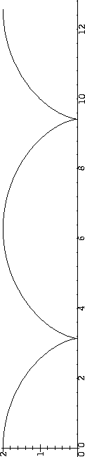
startsection section10mm-.5 Discussion 8 Further Exploration of Parametric Curves

 This is a L^ATEXversion of a Maple worksheet. The worksheet is available in the directory /home/stu/courses/math141.

startsection subsection10mm.5 Introduction In this discussion we continue our exploration of parametric curves using Maple. In the first exercise we consider the motion of a fixed point on a wheel as the wheel rolls in a straight line. In the second and third exercise we consider the motion of an object near the surface of the earth which is launched with an initial velocity and then is subject to the forces of gravity and air resistance. Each of these motions occurs in a plane and we will use the Maple command plot to plot the curve which represents the motion.

startsection subsection10mm.5 Exercises Be sure to load the Maple package plots before you begin your Maple session.

1.

Let us consider a particular example of motion in the plane. The motion can be described as follows: Consider a wheel of radius 1 that rests on the x-axis and rolls without slipping in the positive direction along the x-axis with unit speed. If we mark a point on the wheel, it will trace a curve in the plane as the wheel rolls. This curve is called a cycloid. If we assume that the motion starts with the wheel resting on the origin and that the marked point is at the top of the wheel at the beginning of the motion, the motion is parametrized by

$$\boldsymbol{\alpha}(t) = (t + \sin(t), 1 + \cos(t)).$$

(a)

Use the Maple command plot to plot the image of $\boldsymbol{\alpha}$on the interval $[0,4\pi]$.

(b)

Identify the points on the plot where the marked point is on the ground, is at the same height as the center of the wheel, and is furthest from the ground.

(c)

Determine the time at which the marked point reaches each of the locations you identified in part (b) and the location of the center of the wheel at each of these times.

(d)

Parametrize a circle which represents the wheel when

i.

it is resting on the x-axis at the origin;

ii.

the marked point is first at the level of the center of the wheel;

iii.

the marked point is first on the ground.

In general, how would you parametrize a circle that represents the wheel after it has rolled for t₀ seconds?

(e)

Use the plot command of Maple to plot a circle that represents the wheel when it is in each of the three positions of (d)i-iii.

2.

In this and the next exercise, we want to model the motion of an object near the surface of the earth that is given an initial speed and direction, and is then subject only to the forces of gravity and air resistance or drag. Let us warm up by neglecting drag, which is equivalent to assuming that the object is moving through a vacuum. If a particle is given an initial speed s₀ at an angle $\theta$ from the horizontal, the motion can be parametrized by

$$\boldsymbol{\alpha}(t) = (x_{0} + s_{0}\cos(\theta)t,y_{0} + s_{0}\sin(\theta)t - \frac{9.8}{2}t^{2}),$$

where (x₀,y₀) is the initial position of the object. (Here we are measuring distance in meters and time in seconds.) Let us assume that the object is moving over the surface of the earth, which we assume to be flat and horizontal, and that the initial position is (0,0).

(a)

If we fix the initial speed s₀, for which angle $\theta$will the object travel farthest over the ground? At this angle, how long will the object remain in motion, and how far will the object travel? Explain your answers. (Hint: This is a problem in one variable calculus.)

(b)

Use the Maple command plot to plot the image of $\boldsymbol{\alpha}$ from t=0 to when the object returns to the earth for the angle $\theta_{max}$ of part (a), and the images of $\boldsymbol{\alpha}$ for an angle $\theta$ with $\theta < \theta_{max}$ and $\theta > \theta_{max}$. (Use the value $s_{0} = 10 \mbox{ m/sec}$).

3.

Now let us incorporate drag into our model. Drag is a force that acts opposite to the direction of motion and whose magnitude increases with the speed of the object. The simplest model with drag assumes that the magnitude of the drag force is proportional to the speed of the object. Under this assumption, the motion of the object can be parametrized by

$$\boldsymbol{\alpha}(t) = (x_{0} + \frac{s_{0}\cos(\theta)}{k}... ...\frac{1}{k}(s_{0}\sin(\theta) + \frac{9.8}{k})(1 - e^{-kt}) ),$$

where k is the constant of proportionality. These equations are more complicated than the drag-free equations and it is not possible to determine an exact numerical value for quantities such as the angle that maximizes the horizontal distance travelled by the object. However, we can use Maple to obtain numerical values for quantities of interest to us. Let us try this for a problem from soccer.

  

Figure:

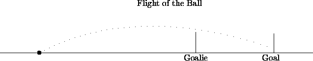
Suppose that an offensive player has broken away from the defenders and only the goalie is between the player and the goal. We would like to know at what angle and what speed the player should kick the ball in order to score a goal by kicking the ball over the goalie's head. The drag coefficient for a soccer ball is approximately .33, so that if we assume that the initial position of the soccer ball is at the origin, the motion of the ball is parametrized by

$$\boldsymbol{\alpha}(t) = (\frac{s_{0}\cos(\theta)}{.33}(1 - e... ...1}{.33}(s_{0}\sin(\theta) + \frac{9.8}{.33})(1 - e^{-.33t}) ).$$

Then in Maple, we can define $\boldsymbol{\alpha}$ by

    alpha:= t -> (s0*cos(theta)/.33*(1 - exp(-.33*t)),-9.8*t/.33 + 
                      (s0*sin(theta) + 9.8/.33)*(1 -exp(-.33*t))/.33;

(In order to use this command, you must first assign numerical values for the initial speed s0 and the angle theta.) Assume that the player is 30 m. from the goal, the goalie is 10 m. from the goal, and that the goalie can deflect the ball if it is less than 2.6 m. from the ground. The goal is 2.44 m. high. Then the image of the flight of the ball, the reach of the goalie and the goal can be plotted with the command

    plot({[alpha(t),t=0..tmax],[20,t,t=0..2.60],[30,t,t=0..2.44]});

where tmax is a constant (tmax =2 will do initially). By experimenting with different values of $\theta$ and s₀ it is possible to find values that will cause the image of the parametric curve to have y coordinate greater than 2.6 when x = 20, so that the ball would pass over the goalie, and to have y coordinate between 0 and 2.44 when x = 30, so that the ball would pass through the goal mouth.

(a)

By experimenting in this manner, determine the minimum speed that is needed to kick the ball over the goalie's reach and score a goal and the angle that should be used with this minimum speed.

(b)

Similarly, determine the maximum speed with which it is possible to kick the ball over the goalie's reach and score a goal and the angle that should be used with this maximum speed.

startsection section10mm-.5 Discussion 9 The Derivative of a Parametrization

 

If the function $\boldsymbol{\alpha}(t)$ is a parametrization of the motion of an object in the plane or in space, then the derivative ${\boldsymbol{\alpha}}'(t)$ is the velocity vector of the motion. That is, for any $t \in (a,b)$, ${\boldsymbol{\alpha}}'(t)$ is a vector which points in the direction of motion and has length equal to the speed of the object at time t. More generally, the vector ${\boldsymbol{\alpha}}'(t)$ is called the tangent vector of the parametrization.

When studying differentiable functions of one variable, y = f(x), we investigated what the derivative of f could tell about the behavior of f. Similarly, in this discussion we will investigate what the derivative of $\boldsymbol{\alpha}$ can tell us about the behavior of $\boldsymbol{\alpha}(t)$. We will focus on two parametrizations we have considered previously, the parametrization of the motion of an object near the surface of the earth which is given an initial speed and direction and the cycloid of Discussion 8..

startsection subsection10mm.5 Exercises

1.

Assume that the parametric curve $\boldsymbol{\alpha}(t) = (x(t),y(t))$ represents the motion of an object in the plane. What can we learn about the motion of the object by examining the velocity vector of the parametric curve?

2.

Let us consider the parametrization of the motion of an object near the surface of the earth which is given an initial speed and direction. If the object is given an initial speed s₀ at an angle $\theta$ from the horizontal, the motion can be parametrized by

$$\boldsymbol{\alpha}(t) = (x_{0} + s_{0}\cos(\theta)t,y_{0} + s_{0}\sin(\theta)t - \frac{9.8}{2}t^{2}),$$

where (x₀,y₀) is the initial position of the object. (Here we are measuring distance in meters and time in seconds.)

(a)

Sketch the path of the object and sketch several velocity vectors on the plot. You should pay attention to both the length and direction of these vectors.

(b)

How do the velocity vectors and speed of the object as it is rising compare to the velocity vectors and speed as it is falling? In particular, how do the velocity vector and speed at a fixed altitude as the object is rising compare to the velocity vector and speed at the same altitude as it falls?

3.

Let us consider the example of the cycloid introduced in Discussion 8. We recall that a cycloid is traced by a point on the edge of a wheel which rolls without slipping along a horizontal axis. If we assume that the wheel has radius 1, that the motion starts with the wheel resting on the origin, and that the marked point is at the top of the wheel at the beginning of the motion, the point traces the parametric curve

$$\boldsymbol{\alpha}(t) = (t + \sin(t), 1 + \cos(t)).$$

Figure is a plot of the parametric curve for t in the interval $[0,4\pi]$.

(a)

Sketch several velocity vectors on the plot of the cycloid, paying particular attention to the length of the vectors.

(b)

Where is the particle moving fastest? Where is it moving slowest? Explain your answer.

(c)

Since the coordinates of the $\boldsymbol{\alpha}(t)$ are differentiable functions, how do you explain the cusps in the cycloid?

  

Figure: The image of $\boldsymbol{\alpha}(t)$ for Exercise 3, $0 \leq t \leq 4\pi$.

startsection section10mm-.5 Discussion 10 Applications of Parametric Curves

 

Our initial motivation for considering parametric curves was to model the motion of an object in the plane or in space. There are, however, a large number of other ``real-world'' events that can be modelled by parametric curves. In Section 2.3 of the text, we investigated three such models. In this discussion, we will study an additional model where the coordinates of the relevant parametric curve do not represent the position of an object in the plane or space. The model we will investigate is for the volume and pressure of a human heart and is an extension of the pump model introduced in Section 2.3. We have included sufficient background material on the model so that the discussion is self-contained.

startsection subsection10mm.5 The Cardiac Cycle Here we investigate a model of the human cardiac cycle that utilizes parametric curves to study the functioning of the heart. It is not possible to obtain a symbolic form for the parametrization of the curve in this case. Nevertheless, it is possible to obtain useful qualitative information from the parametric curve. Before we examine the model, we will provide a brief introduction to heart function. (For further information about this model, see F.C. Hoppensteadt and C.S. Peskin, Mathematics in Medicine and the Life Sciences, Springer-Verlag, 1992, and Leon Glass, et. al., Theory of Heart, Springer-Verlag, 1991.)

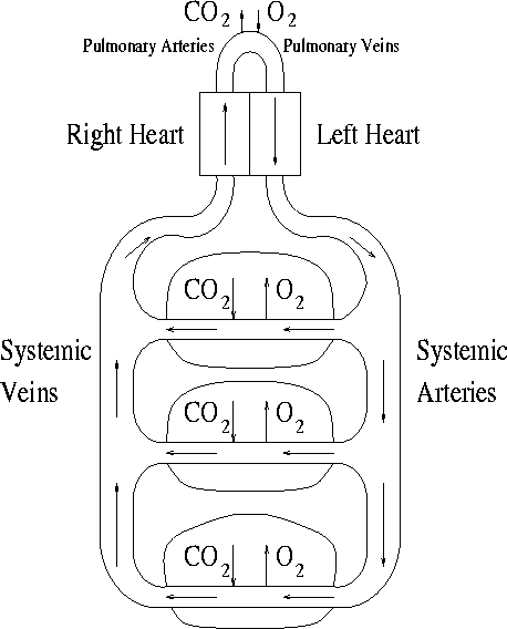
The heart is a muscular, hollow organ that pumps blood through the circulatory system. The right side of the heart pumps blood through the pulmonary arteries to the lungs, where it is oxygenated in the pulmonary capillaries. The oxygen-rich blood returns to the left side of the heart through the pulmonary veins. The left side of the heart pumps blood through the systemic arteries to the entire body. As the blood passes through the systemic capillaries to the systemic veins, the exchange of CO₂ for O₂ occurs. The blood then returns to the right side of the heart through the systemic veins, completing the circulatory loop. (See Figure .)

Since both sides of the heart function in a similar manner during the heart cycle, we will focus on the left heart activity, in particular, on the behavior of the left ventricle as it pumps blood from the pulmonary veins to the systemic arteries. There are two portions to the heart cycle, diastole, when the heart is expanding and filling with blood, and systole, when the heart is contracting and expelling blood. During diastole the mitral valve, which connects the left atrium to the left ventricle is open and blood enters the left ventricle.

  

Figure: A schematic diagram for the human circulatory system.

While this is going on the aortic valve, which connects the left ventricle to the aorta and the systemic arteries, is closed. As the ventricle fills, the pressure in the ventricle increases enough to close the mitral valve, at which time diastole ends and systole begins. The ventricle then contracts, increasing the ventricular pressure until it exceeds the aortic pressure, which opens the aortic valve so that blood can flow into the aorta. When most of the blood is expelled from the ventricle, the aortic valve closes due to the drop in pressure in the ventricle, ending systole. As the heart relaxes, the pressure in the ventricle drops further and the mitral valve reopens, renewing the heart cycle.

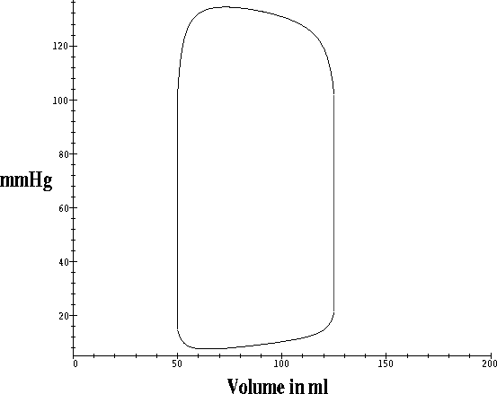
It is natural to use time as a parameter in describing the behavior of the pressure and the volume of the blood in the left ventricle. We will write v(t) for the volume and p(t) for the pressure. Physiologists and cardiologists often study v(t) and p(t)simultaneously using the parametric curve $\boldsymbol{\alpha}(t) = (v(t),p(t))$. If we assume that the heart is beating at approximately 80 heartbeats per minute, then the heart cycle lasts for approximately .75 seconds. Thus we may take the domain for $\boldsymbol{\alpha}(t)$ to be the interval [0,.75]. The following exercises are concerned with the parametric curve $\boldsymbol{\alpha}(t)$.

startsection subsection10mm.5 Exercises Figure is a plot of $\boldsymbol{\alpha}(t)$ for a typical heart cycle. Note that the horizontal axis is the volume axis and the vertical axis is the pressure axis. Volume is measured in milliliters and pressure is measured in millimeters of mercury.

1.

Based upon the above description of the cardiac cycle, label the plot of $\boldsymbol{\alpha}(t)$ with the events of the cycle. In particular, mark where diastole and systole begin and end, where the heart is filling and where the heart is expelling blood. Explain why you labeled the plot in this way. Explain why the plot of $\boldsymbol{\alpha}(t)$ has sides that are vertical.

2.

The left ventricle must create enough pressure to overcome the pressure in the systemic arteries in order to open the aortic valve and expel oxygenated blood into the systemic arteries. Naturally, the greater the arterial pressure, the more difficult it is for the ventricle to pump blood into the arteries. So as the pressure in the systemic arteries increases, the volume of blood that the ventricle is able to pump against this pressure decreases, leaving more blood in the ventricle at the end of systole. Thus the minimum volume of the ventricle during a cycle is an increasing function of the arterial pressure. It has been shown experimentally that this relationship is linear, so we may write

p_a = c (v_min - v₀)

where v₀ is a constant, which is approximately 8 ml on our scale, c is a constant, and p_a is the arterial pressure. The value v_min for a cardiac cycle can be read off the pressure volume plot. Since p_a is the same as the ventricular pressure at the end of systole, it too can be read off the plot of a cardiac cycle. Thus it is possible to determine c from the pressure-volume plot.

Since we know v₀ and can determine c from a pressure-volume plot, we can determine the relation between the pressure at the end of systole and the minimum volume of the ventricle for any cardiac cycle. That is, we can determine the location of the end of systole in the pressure-volume plane: it must lie on the line p = c ( v - v₀). This line is called the end-systolic pressure-volume relation.

  

Figure:

(a)

Based upon the given plot of a cardiac cycle, determine the value of c. Justify the choices of v_min and p_a that you used to determine c.

(b)

Now that you have determined c, it is possible to plot the line p = c(v - v₀) in volume-pressure coordinates, the coordinates of our plot. Superimpose the plot of the end-systolic pressure-volume relation on the given plot of $\boldsymbol{\alpha}(t)$.

3.

Similar to the above straight line that determines the end of systole, there is a curve that determines the end of diastole. This is called the end-diastolic pressure-volume relation. It has been determined experimentally. Although it is not a straight line, it can be given in the form of a function p = f(v) that satisfies three properties

• f(0) = 0.
• f is concave up and increasing.
• f is tangent to $\boldsymbol{\alpha}$ for any pressure-volume parametrization $\boldsymbol{\alpha}(t)$ at the end of diastole.

(a)

Explain how to construct a rough sketch of the end-diastolic pressure-volume relation given these conditions and a cardiac cycle plot.

(b)

Use the cardiac cycle plot given in this discussion to sketch the end-diastolic pressure-volume relation on the same plot that we have been using.

4.

You should now have two plots superimposed on the cardiac cycle plot, a straight line representing the end-systolic pressure-volume relation, and the graph of a function representing the end-diastolic pressure-volume relation.

(a)

Explain how the cardiac cycle plot can be recovered from the end-systolic pressure-volume relation and the end-diastolic pressure-volume relation if the systemic arterial pressure is known.

(b)

Suppose that the systemic arterial pressure decreases by 20 mmHg. How does this shift the cardiac cycle from the given one? Explain your answer and then plot the new cardiac cycle on the original plot.

(c)

Suppose that the systemic arterial pressure increases by 20 mmHg. How does this shift the cardiac cycle from the given one? Explain your answer and then plot the new cardiac cycle on the original plot.

(d)

What is the effect of these changes in arterial pressure on the minimum volume in the heart? What are the physical implications of this?

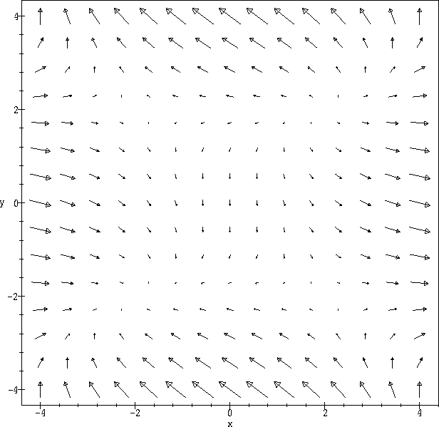
startsection section10mm-.5 Discussion 11 Vector Fields

 

In this discussion we will focus on vector fields in the plane and the flow lines of a vector field.

A vector field in the plane is a function ${\bf F}$ on a region ${\cal D}$ in the plane that assigns a vector to each point in ${\cal D}$, that is, ${\bf F}:{\cal D} \subset {\bf R}^{2} \rightarrow {\bf R}^{2}$. We write

$${\bf F}(x,y) = (u(x,y),v(x,y)),$$

where u(x,y) and v(x,y) are real-valued functions defined on ${\cal D} \subset {\bf R}^2$. Graphically, a vector field on a region ${\cal D}$ is represented by a sketch of the vectors ${\bf F}(x,y)$ with initial point (x,y) for a representative number of points $(x,y) \in {\cal D}$.

A flow line of a vector field ${\bf F}$ is a parametric curve $\boldsymbol{\alpha}:[0,b] \rightarrow {\bf R}^{2}$ whose tangent vector coincides with the vector field ${\bf F}$ at each point of the image of $\boldsymbol{\alpha}$. That is,

$$\boldsymbol{\alpha}'(t) = {\bf F}(\boldsymbol{\alpha}(t)), \ t \in [0,b].$$

In coordinates, if $\boldsymbol{\alpha}(t) = (x(t),y(t))$, then

$$(x'(t), y'(t)) = (u(x(t), y(t)),\ v(x(t),y(t))).$$

Intuitively, if the vector field represents a fluid flow in the plane, a flow line would represent the motion of a particle in this flow. startsection subsection10mm.5 Exercises

1.

Describe a procedure you could use to sketch flow lines for a vector field in the plane given a graphical representation.

2.

Attached are the plots of several vector fields. The symbolic form for the vector field is given on the plot. For each vector field,

• Determine the points where the vector field is zero by solving the equations u(x,y) =0 and v(x,y)=0 for x and y. These are called the critical points of the vector field.
• Sketch several different flow lines on the plot.
• Describe the family of flow lines for each vector field.

  

Figure: The vector field ${\bf F}(x,y)= (-y,x)$ for Exercise 2 of Discussion 11.

  

Figure: The vector field ${\bf F}(x,y)= (y,x)$ for Exercise 2 of Discussion 11.

  

Figure: The vector field ${\bf F}(x,y)= (4y + 2x,-2x -2y)$ for Exercise 2 of Discussion 11.

  

Figure: The vector field ${\bf F}(x,y)=(2x + y,x + 2y)$ for Exercise 2 of Discussion 11.

  

Figure: The vector field ${\bf F}(x,y)= (x^{2} - y^{2},y^{2}-4)$ for Exercise 2 of Discussion 11.

  

Figure: The vector field ${\bf F}(x,y)= (\sin(x-y),\cos(x+y))$ for Exercise 2 of Discussion 11.

startsection section10mm-.5 Discussion 12 Critical Points of Vector Fields

 

This is a L^ATEXversion of a Maple worksheet. The worksheet is available in the directory /home/stu/courses/math141.

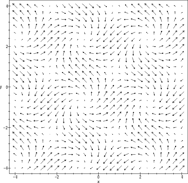
startsection subsection10mm.5 Introduction In the previous discussion we introduced and began to analyze vector fields. We located the critical points of the vector field, and sketched flow lines. If we think of the vector field as modelling the flow of a fluid, a flow line represents the motion of a particle in the flow. In this discussion, we will use Maple to plot vector fields and to compute their flow lines. We will then analyze these plots in order to classify the critical points of the vector field.

startsection subsection10mm.5 Flow Lines and Critical Points A flow line for the vector field ${\bf F}(x,y) = (u(x,y),v(x,y))$ is a function $\boldsymbol{\alpha}$ that satisfies $\boldsymbol{\alpha}'(t) = {\bf F}(\boldsymbol{\alpha}(t))$. Equivalently, $\boldsymbol{\alpha}(t) = (x(t),y(t))$ is a flow line of ${\bf F}$ with initial point (x₀,y₀) if x(t) and y(t) satisfy the system of differential equations

$$\begin{eqnarray*}x'(t) &=& u(x(t),y(t)) \\ y'(t) &=& v(x(t),y(t)), \end{eqnarray*}$$

subject to the initial conditions x(0) = x₀ and y(0) = y₀.

In general, this system may be difficult or impossible to solve algebraically. We can, however, use Maple to compute an approximate solution and plot the solution curve. The technique Maple uses is a graphical integration technique which is similar to the technique we used to sketch flow lines by hand. At the initial point, Maple moves a short distance in the direction of the vector field at that point to a second point and then repeats the process. The advantage of using Maple is that the computer can repeat the process for a large number of points that are close together, thus producing a smoother and more accurate flow line. A point (x₀, y₀) is a critical point of the vector field ${\bf F}$ if ${\bf F}(x_0,y_0) = (0,0)$. Based upon the plots from the previous discussion, we can see that there are two distinct types of critical points: those with the property that every flow line that begins near the critical point, remains near the critical point, which are called stable; and those that do not have this property, which are called unstable. In this discussion, we will use Maple to plot flow lines near a critical point in order to determine whether it is stable or unstable. startsection subsection10mm.5 Plotting Vector Fields and Flow Lines in Maple

We will use the Maple commands fieldplot to plot a vector field in the plane and DEplot to plot the flow lines of a vector field. In this section we will give a brief description of these commands, but, as usual, you should consult the Maple Help utility for more complete information.

The command fieldplot is in the package plots and the command DEplot is in the package DEtools, so you must load these packages before you can plot the vector fields. To do so, enter the following commands

      > with(plots):
      > with(DEtools):

fieldplot

To use the fieldplot command to plot the vector field ${\bf F}$, we can either enter the expression for ${\bf F}$ directly into the command; or we can use the := construction to define ${\bf F}$ and then enter ${\bf F}(x,y)$ into the fieldplot command. Here we demonstrate the second use.

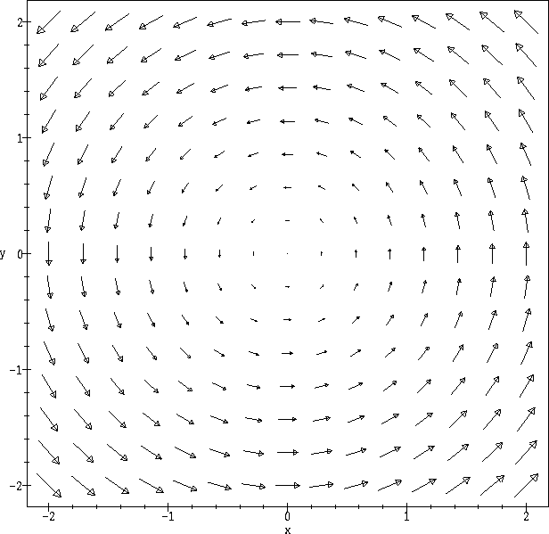
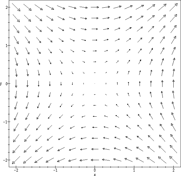
As an example, let us define the vector field ${\bf F}(x,y) = (x-y,x+y)$ in Maple:

      > F:=(x,y)->[x -y, x + y];

To plot the vector field ${\bf F}$ on $[a,b] \times [c,d]$ , use the command

      > fieldplot(F(x,y), x = a..b, y=c..d, arrows = SLIM, grid = [#,#]);

where ${\bf F}(x,y)$ is the pre-defined vector field. The option arrows = SLIM sets the style of the vectors and the option grid = [#, #] sets the number of vectors that are plotted. The default value for the arrows option is arrows = THIN and the default grid size is [20,20]. In order not to clutter the image, fieldplot scales the length of the vectors in the image. The direction of the displayed vectors is correct, but only their relative lengths are correct. That is, longer vectors appear longer and shorter vectors appear shorter.

Here is an implementation of the command without changing the default choices for arrows and grid.

      > fieldplot(F(x,y),x=-2..2,y=-2..2);

Here is an implementation of the command with these defaults reset.

      > fieldplot(F(x,y),x=-2..2,y=-2..2,arrows=SLIM,grid=[10,10]);

DEplot

The Maple command DEplot is used to plot flow lines of a vector field. In fact, it solves the differential equations that define the flow lines of the field for a list of initial points, and then plots the corresponding solutions. Let us begin with the differential equations that define the flow lines of

$${\bf F}(x,y) = (u(x,y),v(x,y)).$$

The differential equations are:

$$\begin{eqnarray*}x'(t) &=& u(x(t),y(t)) \\ y'(t) &=& v(x(t),y(t)). \end{eqnarray*}$$

We can use the built-in differentiation command, diff, to evaluate the derivatives. As we did above, we define an expression for these equations, so that we do not have to enter them more than once for each function. The correct format for the expression is:

      {diff(x(t),t) = u(x,y) , diff(y(t),t) = v(x,y) }

Let us define this in Maple for the vector field ${\bf F}(x,y) = (x-y,x+y)$ that we used above.

      > eqns:={diff(x(t),t)= x(t)-y(t), diff(y(t),t)=x(t)+y(t)};

We must also specify the initial points for the flow lines. This should be a Maple list of ordered pairs, which takes the form:

      {[x(0)=x1,y(0)=y1],[x(0)=x2,y(0)=y2], ... , [x(0)=xk,y(0)=yk]}

Again, we define this using the := construction. Putting this together with DEplot, we have an example of plotting flow lines. We will explain the options after the command:

      > inits:={[x(0)=1,y(0)=0],[x(0)=2,y(0)=0],[x(0)= 0,y(0)=1.5]}:
      > DEplot(eqns,[x,y],t=0..1,inits,x=-3..3,y=-3..3,stepsize=.1,arrows=SLIM);

[x,y

] Specifies the dependent variables to be plotted.

t =a..b

This specifies the range for t, which is domain of the flow line.

x=c..d,y=e..f

These ranges specify the size of the rectangle that is displayed. Any portion of a flow line which exceeds this range will not be plotted.

stepsize =s

This specifies the size of the step in the graphical integration routine. A smaller stepsize will give a smoother flow line but it will also take longer to compute the flow line. In general, a stepsize of .1 or .2 is acceptable.

arrows = SLIM

This setting causes Maple to plot a direction field with two-sided arrowheads. By omitting the arrows options, Maple plots with one-sided arrowheads. The value NONE causes Maple to plot the flow lines but no vectors. Note that DEplot produces normalized vectors which all have the same length. They point in the same direction as the vector field, but do not reflect the lengths of the vectors in the field. Thus they indicate the direction of the flow line but not the speed of the flow line.

To plot the flow lines and scaled vectors, it is necessary to combine the fieldplot and DEplot commands with the display command. Here is how to do it:

      > inits:={[x(0)=1,y(0)=0],[x(0)=2,y(0)=0],[x(0)= 0,y(0)=1.5]}:
      > A:=DEplot(eqns,[x,y],t=0..1,inits,x=-3..3,y=-3..3,stepsize=.1,
               arrows=NONE):
      > B:=fieldplot(F(x,y),x=-3..3,y=-3..3,arrows=SLIM,grid=[15,15]):
      > display([A,B]);

startsection subsection10mm.5 Exercises Before beginning these exercises, if you have not already done so, load the Maple packages plots and DEtools using the commands

      > with(plots):
      > with(DEtools):

1.

For each of the following vector fields:

i.

Find the coordinates of the critical points by hand.

ii.

Use the Maple command fieldplot to plot the vector field.

iii.

Using the plot of the vector field, choose several initial points near each critical point and use the Maple command DEplot to plot the flow lines for these initial points.

iv.

Based upon the behavior of the flow lines near a critical point, determine whether it is a stable or unstable critical point. Explain why the critical point is stable or unstable.

Note: The Maple commands you need are given with the vector field in (a). Only the Maple vector field definition is given in the following parts. For the remaining parts, you should copy the commands from (a), change eqns and inits, and the plot range and time range (in DEplot) options, then execute the commands. You may also want to change the grid to display more vectors or fewer vectors.

(a)

${\bf F}(x,y) = (-x-2y,2x+y).$
The vector field definition in Maple is:

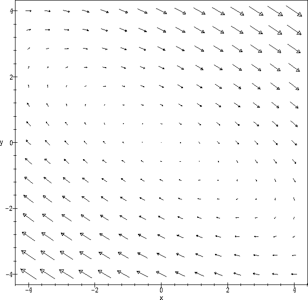
      > F:=(x,y) -> [-x-2*y,2*x+y]:

The following command plots F on the rectangle $[-3,3]\times[-3,3]:$

      > fieldplot(F(x,y),x=-3..3,y=-3..3,arrows=SLIM);

The following commands, define the equations, the list of initial conditions, and plots the flow lines.

NOTE: You must enter your initial conditions (as above) in order to execute DEplot.

      > eqns:={diff(x(t),t)= -x(t)-2*y(t), diff(y(t),t)=2*x(t)+y(t)}:
      > inits:={[x(0)= ?? ,y(0)= ?? ] }:
      > DEplot(eqns,[x,y],t=0..1,inits,x=-3..3,y=-3..3,stepsize=.1,
              arrows=SLIM);

The following commands combine the scaled vector field plot from fieldplot with the flowlines from DEplot:

      > A:=fieldplot(F(x,y),x=-3..3,y=-3..3,arrows=SLIM,
               grid=[10,10]):
      > B:=DEplot(eqns,[x,y],t=0..1,inits,x=-3..3,y=-3..3,stepsize=.1,
              arrows=NONE):
      > display([A,B]);

(b)

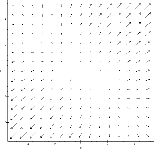
${\bf F}(x,y) = (-x + y, -x - y)$.

      > F:=(x,y)->[-x+y,-x-y];

(c)

${\bf F}(x,y) = (.8x - .6y, -.6x - .8y)$

      > F:=(x,y)->[.8*x - .6*y, -.6*x - .8*y];

(d)

${\bf F}(x,y) = (x^2 -1, y^2 -1)$. Use the domain $[-3,3] \times [-3,3].$

      > F:=(x,y)->[x^2 -1, y^2 -1];

(e)

${\bf F}(x,y)= (\sin(x-y),\cos(x+y))$. Use the domain $[-4,4] \times [-4,4]$. This is one of the vector fields you looked at in the previous discussion. How do your flow lines compare compare to the computer generated flow lines?

      > F:=(x,y)->[sin(x-y), cos(x+y)];

(f)

${\bf F}(x,y) = (y, 16 \sin x + .0025 \cos x \sin y)$. Use the domain $[-5,5] \times [-10,10]$

      > F:=(x,y)-> [y, 16*sin( x) + .0025*cos(x)*sin(y)];

2.

It should be clear by now that there are several different possible behaviors for flow lines near a stable critical point and for flow lines near an unstable critical point. Based upon the examples that you have considered, describe the different behaviors for flow lines near stable and unstable critical points. Further, for each of the critical points of the vector fields of Exercise 1, decide which of your descriptions applies to the given critical point.

startsection section10mm-.5 Discussion 13 Vector Fields As Models

 

This discussion consists of three extended modelling assignments that are intended to provide the opportunity to work with and modify more involved models than have been developed so far. The first assignment considers two physical models, the damped pendulum and the bead on the wire, which build on the simple pendulum model developed in Section 2.5 of the text. The second assignment considers two population models, a predator-prey model and a competition model, which build on the predator-prey model developed in Section 2.5 of the text. The third assignment considers two models for the spread of an epidemic, an SIR model and an SI model with reinfection, which build on the SIR model developed in Section 2.3 of the text.

Each assignment requires you to use the computer. In particular, you should be familiar with the Maple commands for plotting vector fields and their flow lines that were introduced in the previous discussion.

startsection section10mm-.5 Discussion 13 A. Physical Models

 

startsection subsection10mm.5 The Damped Pendulum In the text we investigated two mathematical models for the simple pendulum, first using parametric curves in Section 2.1 and then using vector fields and flow lines in Section 2.5. Here we want to use vector fields and flow lines to construct a model for the motion of a pendulum that incorporates a second force in addition to the force of gravity.

Recall that a simple pendulum consists of a mass concentrated at a point that is suspended from a massless cord or rod which is free to swing without friction in a vertical plane. We saw that x(t), the displacement of the pendulum along its arc, satisfies the differential equation

$$x''(t) = -g \sin(\frac{x(t)}{l}),$$

where g is the acceleration due to gravity and l is the length of the rod. In Section 2.5 of the text, we showed how to model the motion of this pendulum by flow lines of the vector field

$${\bf F}(x,v)=(v,-g\sin(\frac{x}{l}))$$

in the phase plane of the pendulum, whose coordinates are the angular position and angular velocity of the pendulum. A flow line of this vector field is a called a phase-plane trajectory of the pendulum. This is a parametric curve $\boldsymbol{\alpha}(t) = (x(t),v(t))$, where x(t) is the displacement of the pendulum along the arc at time tand v(t) = x'(t) is the velocity of the pendulum at time t. Since $\boldsymbol{\alpha}$ is a flow line of ${\bf F}$,

$$\boldsymbol{\alpha}'(t) = (x'(t), x''(t)) = (v(t), - g\sin(\frac{x(t)}{l})).$$

Now let us consider a more realistic model that incorporates a force which dissipates the energy of the pendulum, for example, friction. (See Serway, Physics for Scientists and Engineers, p. 341.) Any such force is called a damping force and we say that the motion of the pendulum is damped. A damping force acts in a direction opposite to the motion of the pendulum and usually increases with the speed of the pendulum. The simplest example of a damping force is one that is proportional to the speed of the pendulum. In this case, Newton's second law for the component of force in the direction of motion takes the form

$$F = ma = -mg\sin(x/l) - kv,$$

where k >0 is a constant of proportionality. Since v'(t) = a(t), we can rewrite this single second order equation as a system of first order equations in x and v,

$$\begin{eqnarray*}x'(t) & = & v(t)\\ v'(t) & = & -g\sin(x(t)/l) - \frac{k}{m}v(t). \end{eqnarray*}$$

The corresponding vector field ${\bf F}$ is

$${\bf F}(x,v) = (v,-g\sin(\frac{x}{l}) - \frac{k}{m}v).$$

A flow line of ${\bf F}$ with initial point (x₀,v₀)corresponds to the motion of the damped pendulum when its initial angular displacement x₀ and its initial angular velocity is v₀.

startsection subsection10mm.5 Exercises -- The Damped Pendulum Before beginning these exercises, load the Maple packages plots and DEtools.

Assume the length of the rod is 1 meter so the displacement x is equal to the angular displacement of the pendulum from the vertical and that m = 1. Use $g = 9.8\mbox{ m/sec}^2$.

1.

Compute the critical points of ${\bf F}$ by hand. What is the position of the pendulum corresponding to each of these points? Do you expect these points to be stable or unstable? How would you expect the flow lines to behave near these points?

2.

Set k = 1 and use the Maple commands fieldplot and DEplot to determine the types of the critical points of ${\bf F}$. Explain your answer in terms of the flow lines of ${\bf F}$. Describe the behavior of the pendulum that is represented by each of these flow lines.

3.

Let us use our model to analyze the motion of the pendulum as we change its initial velocity. In particular, suppose we consider the motion of the pendulum that occurs when the pendulum is set in motion with velocity v₀ when the initial angle x₀ = 0. Use the model to describe the behavior of the pendulum for the different motions that arise as v₀ increases without bound. Begin with the case v₀= 0. In particular, what qualitative changes occur in the behavior of the pendulum as you choose larger values for v₀.

4.

Now let us investigate the effect of changing the magnitude of the damping force. How would you expect the motion of the pendulum to change if

(a)

the damping coefficient k is increased?

(b)

the damping coefficient k is decreased?

Justify your answers by analyzing the flow lines and critical points of the vector field ${\bf F}$ for different values of k. Explain how these plots support your answers.

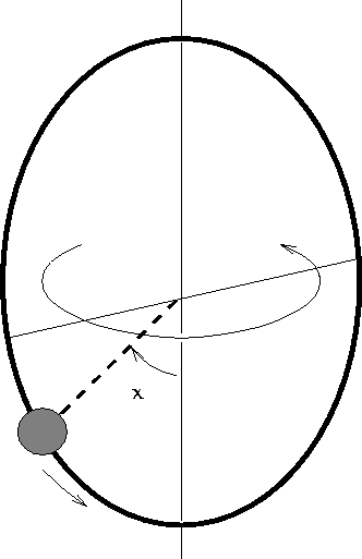
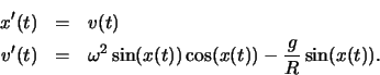
startsection subsection10mm.5 A Bead on a Rotating Wire Here we consider a different mechanical system that can be modelled by the flow lines of a vector field. The system consists of a circular wire of radius R and a bead of mass m that is attached to the wire, but is allowed to move along the wire. (See Figure .) The wire lies in a vertical plane and rotates about a vertical axis at a constant angular speed $\omega$. As the wire rotates, the bead moves along the wire subject to the force of gravity, the force that constrains it to remain on the wire, and friction. We want to investigate the motion of the bead and understand how it depends on the angular speed of the rotating wire. We will begin by considering the case of the frictionless wire. (For further discussions of this model, see Woodhouse, Introduction to Analytical Dynamics, Oxford University Press, p. 18, and Marsden and Ratiu, Introduction to Mechanics and Symmetry, Springer-Verlag, 1994, p. 76.)

  

Figure: A bead on a vertical rotating wire.

We will denote the angular position of the bead on the wire by x, with x=0 corresponding to the bottom of the wire and $x= \pi$ and $x = -\pi$ corresponding to the top of the wire, which both lie on the axis of rotation. When Newton's second law is applied to this system, one obtains the equation

$$x''(t) = \omega^{2} \sin(x(t))\cos(x(t)) - \frac{g}{R}\sin(x(t)),$$

for the angular acceleration of the bead, where g is the acceleration due to gravity. As we did for the motion of the pendulum, we will replace this equation by a pair of equations in the angular position x(t) and the angular velocity v(t) of the bead on the wire. We obtain the following pair of differential equations

$$\begin{eqnarray*}x'(t) & = & v(t)\\ v'(t) & = & \omega^{2}\sin(x(t))\cos(x(t)) - \frac{g}{R}\sin(x(t)). \end{eqnarray*}$$

We will then model the motion of the bead on the rotating wire by the flow lines of the vector field

$${\bf F}(x,v) = (v,\omega^{2}\sin(x)\cos(x) - \frac{g}{R}\sin(x)).$$

A flow line of ${\bf F}$ with initial point (x₀,v₀) will model the motion of the bead when it is given an initial angular velocity of v₀ at an initial angular position of x₀.

startsection subsection10mm.5 Exercises -- Bead on a Rotating Wire

1.

Find the critical points of the vector field ${\bf F}$. Do the critical points depend on the speed of rotation of the wire $\omega$? Explain. What is the position of the bead corresponding to each of these points? Do you expect these points to be stable or unstable? How would you expect the flow lines to behave near these points.

2.

Let us assume that R=.5. Suppose further that the speed of rotation $\omega = 1$. Use the Maple commands fieldplot and DEplot to determine the types of the critical points of ${\bf F}$. Explain your answer in terms of the flow lines of ${\bf F}$. Describe the behavior of the bead that is represented by each of these flow lines.

3.

Let us use our model to analyze the motion of the bead as we change the speed of rotation $\omega$. Suppose that $\omega$ is allowed to increase. Investigate the behavior of the bead by plotting ${\bf F}$and several of its flow lines for different values $\omega > 1$. (You may want to fix a collection of initial points that you use for the different values of $\omega$.) For each $\omega$, describe the behavior of the bead that is represented by each of the flow lines. Be sure to pay attention to the changes, if any, in the motion of the bead for a given initial position and velocity as $\omega$ is increased.

4.

Now let us incorporate the resistive force of friction into our model. Friction acts in a direction opposite the direction of motion of the bead. Let us suppose that friction is proportional to the angular velocity of the bead. Then Newton's second law yields the second order equation

$$x''(t) = \omega^{2} \sin(x(t) )\cos(x(t) ) - \frac{g}{R}\sin(x(t) ) - \frac{k}{m}x'(t)$$

for the angular acceleration of the bead, where the constant of proportionality k is positive. It follows, as above, that the we can model the motion of the bead by a flow line of the vector field

$${\bf F}(x,v) = (v,\omega^{2}\sin(x)\cos(x) - \frac{g}{R}\sin(x) - \frac{k}{m}v).$$

Let us assume that R =.5 as above and that m=1. How would you expect the motion of the bead to change for a given angular speed of rotation $\omega$ if resistive force of friction is not too large, that is, k < 1? Justify your answer by analyzing the flow lines and critical points of the vector field ${\bf F}$ for different values of $\omega$ that you considered above. Explain how these plots support your answers.

startsection section10mm-.5 Discussion 13 B. Models of Interacting Populations

 

In Section 2.5 of the text, we introduced a vector field to model a system consisting of two populations which interacted as predator and prey. This model is called the Predator-Prey model. In this discussion, we would like to modify this model to construct more realistic models of interacting populations. startsection subsection10mm.5 Predator-Prey With Fishing The predator-prey model described in the text is based upon several assumptions. First we assumed that in the absence of predators, the rate of growth of the prey is proportional to the number of prey, that is, we assumed that the growth of the prey is exponential. Second, we assumed that the number of interactions between predator and prey is proportional to the product of the two populations, and that the rate of growth of the prey is decreased by a rate proportional to the number of interactions and the rate of growth of the predators is increased by a rate proportional to the number of interactions. Finally, we assumed that there are no other external factors influencing the rates of growth of the predator and prey populations. Under these assumptions, if x represents the prey population and y represents the predator population, then the rates of change of the prey and predator populations are modelled by

$$\begin{eqnarray*}x'(t)& = &ax(t) - bx(t)y(t) \\ y'(t)& = & -cy(t) + dx(t)y(t), \end{eqnarray*}$$

where a, b, c, and d are positive constants.

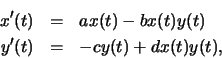
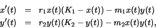
As a first example, we would like consider a model that incorporates an external factor. In the particular example we want to present a model where the predators are sharks (selachians) and the prey are all other fish, and both populations are subject to fishing. Thus xrepresents the size of the fish population and y represents the size of the shark population. In the text Differential Equations and Their Applications, M. Braun describes the observations of an Italian biologist, Umberto D'Ancona who in the 1920's noticed that there had been a substantial change in the shark and fish populations in the Mediterranean for the years 1915 through 1919. D'Ancona suspected that this change could be attributed to the lack of fishing during World War I, but he was unable to completely explain the changes. He asked the mathematician Vito Volterra to develop a mathematical model which would explain these changes. The model we will be working with is the predator-prey model developed by Volterra. (See Braun's text for further information about the observations of D'Ancona and predator-prey models.)

We must modify the standard predator-prey model to include the effect of fishing on both populations. Clearly, fishing decreases the rate of growth of both populations in proportion to the size of the population. Volterra assumed that the constant of proportionality would be the same in both populations. So we add a negative fishing term of the form -mx or -my to the rate of change of the populations x and y respectively. We then have

$$\begin{eqnarray*}x'(t)& = &ax(t) - mx(t) - bx(t)y(t) \\ y'(t)& = & -cy(t) - my(t) + dx(t)y(t), \end{eqnarray*}$$

where a, b, c, d, and m are positive constants.

Thus we will model the behavior of the shark and fish populations by the flow lines of the vector field

$${\bf F}(x,y) = (ax - mx - bxy, -cy -my + dxy).$$

A flow line $\boldsymbol{\alpha}$ of ${\bf F}$ starting at the point (x₀,y₀) will correspond to the behavior of the populations under the assumption that there are initially x₀ fish and y₀ sharks.

startsection subsection10mm.5 Exercises -- Predator-Prey With Fishing

Before beginning these exercises, load the packages plots and DEtools.

Let ${\bf F}(x,y) = (ax - mx - bxy, -cy -my + dxy)$.

1.

We saw in the previous discussion that the critical points of a vector field correspond to solutions which do not change in time. Compute the critical points of ${\bf F}$ by hand.

2.

Use the fieldplot command of Maple to plot ${\bf F}$ with a = 2.5, b = 1, c = 2, d = 1, and m = 1.

(a)

What are the critical points of this vector field?

(b)

Use the DEplot command to plot several flow lines of the vector field. Describe what happens to the fish and shark populations over time for these flow lines. Describe how the flow lines change if you use initial points closer to the critical point. What happens if the initial points are farther away from the critical point?

3.

Now we want to explore what will happen to the populations if we decrease the amount of fishing. In order to model the decrease in fishing we will change m from 1 to .5.

(a)

Describe in general terms what you would expect to happen to the shark and fish populations over time if fishing is decreased.

(b)

Compute the new critical points of this vector field by hand. How does the decrease in fishing change the critical point?

(c)

Use the Maple commands fieldplot and DEplot to investigate the flow lines of this vector field. Use the same initial points as you did in Exercise 2b. How do these flow lines compare to the flow lines you generated in Exercise 2?

(d)

The initial point of a flow line of this vector field represents the size of the populations of fish and sharks at the time that fishing is decreased. Use the Maple command DEplot to plot flow lines which would correspond to beginning the decrease in fishing at points where the fish and shark populations are both low, both high or one low and one high. Does the effect of decreased fishing change depending upon the relative size of the populations when fishing is decreased?

(e)

In general, how does a decrease in fishing affect the populations of fish and sharks? Do you find these results as surprising as D'Ancona did?

startsection subsection10mm.5 Competing Populations

We now want to shift our point of view and consider a model of two populations which are competing for the same resource. We assume that this resource is available in fixed quantities so the rate of growth of each population is effected by the size of the population and the size of the competing population. Suppose that x and y are functions which represent the size of each population at time t. The rate of growth of a population which is dependent upon limited resources is modelled by an equation of the form

x'(t) = rx(t)(K- x(t)),

where r and K are positive constants. This equation is called the logistic equation. We assume that in the absence of a competing population, the rate of growth of each population is modelled by a logistic equation. That is,

$$\begin{eqnarray*}x'(t) &= &r_1 x(t)(K_1-x(t)) \\ y'(t)& = &r_2y(t)(K_2-y(t)), \end{eqnarray*}$$

where r₁, r₂, K₁, and K₂ are positive constants. In the presence of competitors, the rate of change of each population would be decreased by an amount proportional to the product of the two populations. Thus the rates of change of competing populations can be modelled by the equations:

$$\begin{eqnarray*}x' (t)&= &r_1x(t)(K_1-x(t)) - m_1 x(t)y(t) \\ y' (t)&= &r_2y(t)(K_2-y(t)) - m_2 x(t)y(t), \end{eqnarray*}$$

where m₁, and m₂ are also positive constants. The corresponding vector field is

$${\bf F}(x,y) = (r_1x(K_1-x) - m_1 xy, r_2y(K_2-y) - m_2 xy).$$

If $\boldsymbol{\alpha}(t) = (x(t),y(t))$ is a flow line of ${\bf F}$ with initial point (x₀, y₀), $\boldsymbol{\alpha}$ represents the evolution of the two populations assuming that initial there are x₀ and y₀ members of each of the competing populations.

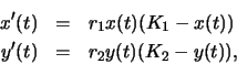
In the exercises below, we will use this model to study the long term effects of competition. Ecologists have observed that generally in ecological systems, if two populations are competing for the same resource, one population eventually dies out. In 1966, P. DeBach stated the following: ``Different species which co-exist indefinitely in the same habitat must have different ecological niches ...'' This statement is known as the competitive exclusion principle. (For further information about this model and the competive exclusion principle see An Introduction in Mathematical Ecology by E.C. Pielou.) By varying the parameters m₁ and m₂ in the model, we would like to determine if the model predicts the competitive exclusion principle.

startsection subsection10mm.5 Exercises -- Competing Populations Before beginning these exercises, load the packages plots and DEtools. In order to simplify the model, we will assume that r₁, r₂, K₁, and K₂ are equal to 1.

1.

Let ${\bf F}(x,y) = (x(1-x)-m_1xy, \; y(1-y)-m_2xy)$.

(a)

Compute the critical points of ${\bf F}$ by hand. (Note: There are 4 critical points.)

(b)

Since x and y represent populations, we will restrict our attention to critical points and flow lines with x>0 and y>0. What are the critical points of ${\bf F}$ satisfying these criteria?

2.

Use the fieldplot command of Maple to plot ${\bf F}$ with m₁ = 1.5 and m₂ = .5.

(a)

What are the critical points of this vector field?

(b)

Use the DEplot command to plot several flow lines of this vector field and determine the types of critical points this vector field has. Describe what happens to the competing populations over time as we follow these flow lines. What is the long term behavior of the system represented by this vector field?

3.

Now let us investigate the effect of changing the parameters m₁ and m₂ on the long term behavior of the system.

(a)

Repeat question 2 for different values of m₁ and m₂. Try to investigate as many different cases as possible. (Hint: Based upon your computations of the critical points, it is clear that the values m₁ = 1 and m₂ = 1 are values which signal a change in the behavior of the system. Be sure to include examples where the values of m₁ and m₂ are greater than 1 and examples where these values are less than 1. )

(b)

Based upon your investigations in part (a), generally describe the long term behavior of this model. Does this model predict the principle of competitive exclusion?

startsection section10mm-.5 Discussion 13 C. Epidemic Models

 

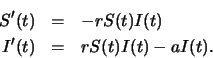
startsection subsection10mm.5 SIR Model In Section 2.3 of the text we introduced the SIR model for the spread of an epidemic and used parametric curves to model a particular epidemic. Here we would like to use vector fields to further explore the SIR model. (See J.D. Murray, Mathematical Biology, Springer-Verlag, 1993, for a more detailed study of the SIR and related models).

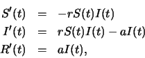
The SIR model for an epidemic divides a population into three groups, the susceptible population, the infected population, and the recovered population, which we will denote by S, I, and R. Initially, we will assume that the size of the population is fixed, so that S + I + R = N is constant. A person who has not yet had the disease is considered to be susceptible; a susceptible person can become infected through contact with an infected person; and an infected person recovers and is henceforth assumed to be immune. In Section 2.3 of the text, we derived equations for the rates of change of these populations based upon the assumptions that the susceptible population decreases, and therefore the infected population increases, at a rate proportional to the number of contacts between the susceptibles and infectives, and that the infected population decreases, and therefore the recovered population increases, at a rate proportional to the size of the infected population. We obtained the equations

$$\begin{eqnarray*}S'(t)& =& -rS(t)I(t)\\ I'(t)&= & rS(t)I(t) - aI(t)\\ R'(t)& = & aI(t), \end{eqnarray*}$$

where r is the rate of infection and a is the rate of recovery, $0 < r,\ a< 1$. Since the size of the population is assumed to be fixed, R is determined by S and I, and we need only determine the evolution of S and I in order to determine the state of the system. Moreover, S' and I' do not depend on R, so it suffices to consider only the first two equations,

$$\begin{eqnarray*}S'(t)& =& -rS(t)I(t)\\ I'(t)&= & rS(t)I(t) - aI(t). \end{eqnarray*}$$

Thus we will model the spread of the epidemic by the flow lines of the vector field

$${\bf F}(S,I) = (-rSI, rSI - aI).$$

A flow line $\boldsymbol{\alpha}$ of ${\bf F}$ starting at the point (S₀,I₀)will correspond to the spread of the epidemic under the assumption that initially there are S₀ susceptibles and I₀ infectives.

startsection subsection10mm.5 Exercises -- SIR Model Be sure to load the packages plots and DEtools before you begin the Maple portions of the exercises.

1.

Assume, as above, that $0< a,\ r < 1$ are constants and $S_{0}, \ I_{0} > 0$.

(a)

Does the vector field ${\bf F}$ have any critical points in the first quadrant in the SI-plane? Does your answer depend on the values of the constants a and r? If there are critical points, find them.

(b)

What is the importance of your answer to (a) for the behavior of an infection?

2.

It is natural to ask under what circumstances an infection will spread so that the number of infectives increases, which we will take to be the definition of an epidemic. Let S₀ denote the initial population of susceptibles and I₀ denote the initial population of infectives.

(a)

For which values of S₀ and I₀ will the infection spread? For which values of S₀ and I₀ will the infection not spread? (Hint: Think about I'.) Explain your answer.

(b)

If the infection does not spread initially, will I continue to decrease until the infection dies out? Explain your answer.

(c)

If the infection spreads initially, will I continue to increase until there are no susceptibles left? Explain your answer.

(d)

Choose particular values for r and a and use the command fieldplot to plot ${\bf F}$. (If ${\bf F}$ has critical points in the first quadrant, be sure to choose the domain for your plot to include the critical points.) For which regions in the first quadrant of the SI-plane will an initial value in the region lead to an epidemic? not lead to an epidemic? Shade the regions on a hard copy of the plot and explain your choice based upon your answers to (a), (b), and (c).

3.

In general, an infection can either die out because the number of infectives goes to zero, die out because the number of susceptibles goes to zero, or continue indefinitely with neither the susceptible or infected populations going to zero. Which cases apply to your example from Exercise 2? Do these same cases apply for all a and r? Explain.

startsection subsection10mm.5 SI Model The SIR model can be modified to cover a variety of different scenarios for the spread of an epidemic. Here we will consider the case where having recovered does not confer immunity from the disease. Therefore, the recovereds do not constitute a separate subgroup of the total population and the model has only two populations, the susceptibles and the infectives. In this case, since the population of susceptibles is replenished by recovered infectives, we want to examine this model over a longer time period. As a consequence, we will no longer assume that the total population is constant, and we have

N(t) = S(t) + I(t).

We must now develop new assumptions for the rates of growth of S and of I.

First, let us consider the susceptible population. Since we are interested in a longer time period, we must take into account the birth rates of the susceptible and infected populations. We will assume that both populations produce offspring that are susceptible, but at possibly different rates. Further, the population of susceptibles will increase at a rate proportional to the infected population as infectives recover and move into the susceptible population. As we did above, we will assume that infection is transmitted at a rate proportional to the populations. Thus the rate of change of the susceptible population will be given by an expression of the form

S'(t) = a₁I(t) + bS(t)- rS(t)I(t),

where the constant a₁ reflects both the birth rate of infectives and the rate of recovery of the infectives, and the constant b is the difference between the birth rate and the death rate of the susceptibles, $0 < a_{1}, \ b,\ r < 1$. The infected population should increase at a rate proportional to the infected and susceptible populations as above. In addition, the infected population should decrease by an amount proportional to the infected population, which will account for the recovery of the infectives and for the death of infectives. Thus

I'(t) = rS(t)I(t) - a₂I(t),

where 0 < a₂ < 1.

We will then model the course of the infection by the flow lines of the vector field

$${\bf F}(S,I) = (a_{1}I + bS- rSI,\ rSI - a_{2}I).$$

A flow line $\boldsymbol{\alpha}$ of ${\bf F}$ starting at the point (S₀,I₀)will correspond to the spread of the epidemic under the assumptions that initially there are S₀ susceptibles and I₀ infectives.

startsection subsection10mm.5 Exercises -- SI Model Be sure to load the packages plots and DEtools before you begin the Maple portions of the exercises.

1.

Assume that $0< a_{1},\ a_{2},\ b,\ r < 1$ are constants.

(a)

Does the vector field ${\bf F}$ have any critical points in the first quadrant in the SI-plane? Does your answer depend on the values of $a_{1},\ a_{2},\ b, \mbox{ and }r$?

(b)

If there are critical points, find them.

2.

In order to carry out a graphical analysis of the flow lines of ${\bf F}$, it is necessary to choose particular values for the constants. Let us use the values a₁ = .17, b = .05, r = .01, and a₂ = .4, so that

$${\bf F}(S,I) = (.17I + .05S- .01SI, \ .01SI - .4I).$$

(a)

Based on your calculations in Exercise 1, does this vector field have critical points in the first quadrant? If so, find them.

(b)

Use the Maple command fieldplot to plot the vector field ${\bf F}$. If ${\bf F}$ has critical points, be sure to choose the domain for your plot to include the critical points.

(c)

Based upon your plot of ${\bf F}$, for which regions in the first quadrant of the S-I-plane, will an initial value in the region lead to an epidemic? not lead to an epidemic? Explain your answer.

(d)

Use the Maple command DEplot to plot the vector field ${\bf F}$along with several flow lines of ${\bf F}$. Based upon your plot, describe the long-term behavior of the susceptible and infected populations.

3.

In general, how do infections governed by the SI model differ from those governed by the SIR model? Explain.