The Sequence of Approximations

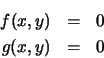
In general, if we are given an initial approximation (x₀,y₀) to a root of a system of equations

$$\begin{eqnarray*}f(x,y) &=& 0\\ g(x,y) &=& 0 \end{eqnarray*}$$

we can produce a sequence of points

$$(x_0,y_0), (x_1,y_1), (x_2,y_2), \dots, (x_i,y_i), (x_{i+1},y_{i+1}),\ldots$$

where the (i+1)^st point in the sequence is obtained from the i^th point by solving the system of linear equations:

$$\begin{eqnarray*}f(x_i,y_i) + \frac{\partial f}{\partial x}(x_i,y_i)(x - x_i) +\... ..._i)(x - x_i) +\frac{\partial g}{\partial y}(x_i,y_i)(y-y_i) &=&0 \end{eqnarray*}$$

If the functions f and g and their partial derivatives satisfy certain conditions on their rate of increase, then it is possible to show that this sequence converges to a root. That is if

$$(x_r,y_r) =\lim_{n \rightarrow \infty}(x_n,y_n),$$

then

$$\begin{eqnarray*}f(x_r,y_r)&=&0\\ g (x_r,y_r)&=&0 \end{eqnarray*}$$

This convergence result is often proven in a course in real analysis. Our focus will be on using this iterative process a finite number of times to produce a numerical approximation to a root and we will explore when this process yields a good approximation. In this next section, we will give Maple procedure for carrying out the iterative process. startsection subsection10mm.5 A Maple Procedure for Newton-Raphson

We can automate the process of computing a finite number of the points in the Newton-Raphson sequence with a Maple procedure. The following is a simple procedure for computing n points of the sequence. The input for the procedure consists of functions f and g, the coordinates of the initial approximation, xinit and yinit, and the number of points to be produced, n. The key part of the procedure is a loop that computes the (i+1)^st point from the i^thpoint. The first line of the loop is the line beginning with the word for and the last line of the loop is the line od: Each time through the loop the equations are redefined and solved for the new basepoint. The results of the calculation are saved in the array pts, which the output of the procedure.

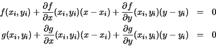
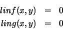
The solution of the equation is expressed in terms of several constants. In order to understand the way the solution is written in the procedure it will help to do some of the algebra by hand. First, the equations linf(x,y) = 0 and ling(x,y) = 0 can be written so that only the terms involving x and y appear on the left hand-side:

    D[1](f)(x0,y0)*x + D[2](f)(x0,y0)*y = -f(x0,y0) 
                   + D[1](f)(x0,y0)*x0 + D[2](f)(x0,y0)*y0
    D[1](g)(x0,y0)*x + D[2](g)(x0,y0)*y = -g(x0,y0) 
                   + D[1](g)(x0,y0)*x0 + D[2](g)(x0,y0)*y0

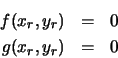
Let us denote the right-hand side of the first equation by rhsf and the right hand side of the second equation by rhsg, so that

    D[1](f)(x0,y0)*x + D[2](f)(x0,y0)*y = rhsf
    D[1](g)(x0,y0)*x + D[2](g)(x0,y0)*y = rhsg

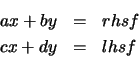
At this point, we should keep in mind that the coefficients of x and y and the right-hand side of each equation are all constants. For the moment, let us replace the coefficients by the letters a, b, c, and d so that the system is given by

$$\begin{eqnarray*}ax + by &=& rhsf\\ cx + dy &=& rhsg \end{eqnarray*}$$

Once the equation is in this form, it a straightforward calculation to show that the system is solved by x and y satisfy:

$$\begin{eqnarray*}x &=& \frac{ rhsf \cdot d - b \cdot rhsg }{ ad - bc}\\ y &=& \frac{ a\cdot rhsg - rhsf\cdot c }{ ad - bc} \end{eqnarray*}$$

(To make sure you understand the procedure you should solve the system and put the solution in this form.)

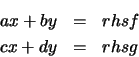
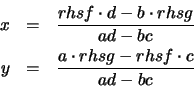
Notice that the solutions for x and y exist as long as the denominator ad-bc is not zero. In other words, before we can compute these solutions, we must make sure that the quantity ad - bc is not zero. This is the role played by the if-then-else-fi in the procedure. If the quantity is zero, the procedure stops and gives as its output the iterate for which this happened. If the quantity is not zero the else portion of the statement is executed. This carries out the calculation of x and y. For more detailed explanation of the syntax that appear in the procedure, click on any of the following hyperlinks: proc, local, for, assign, evalf, if, RETURN.

To load the procedure simply hit the enter key anywhere in the procedure.

    newrap:=proc(f,g,xinit,yinit,n)
    
    local xbase,ybase,i,x,y,a,b,c,d,rhsf,rhsg,pts;
    
    pts:=[xinit,yinit]:
    xbase:=xinit: ybase:=yinit:
    for i from 1 to n do
        x:='x':
        y:='y':
        a:=D[1](f)(xbase,ybase):
        b:=D[2](f)(xbase,ybase):
        c:=D[1](g)(xbase,ybase):
        d:=D[2](g)(xbase,ybase):
    
        if (a*d - b*c = 0) then 
             RETURN(HALT,i)
        else
             rhsf:=-f(xbase,ybase) + D[1](f)(xbase,ybase)*xbase 
                                         + D[2](f)(xbase,ybase)*ybase:
             rhsg:=-g(xbase,ybase) + D[1](g)(xbase,ybase)*xbase  
                                         + D[2](g)(xbase,ybase)*ybase:
             x:=(rhsf*d - rhsg*b)/(a*d - b*c):
             y:=(a*rhsg - rhsf*c)/(a*d - b*c):
             xbase:=evalf(x):ybase:=evalf(y):
             pts:=pts,[xbase,ybase]:
    
    fi: #This ends the if-then-else statment.
    
    od: #This ends the for loop.
    
    RETURN([pts]);
    end:

To apply the procedure, we must define the functions f and g. Here we use the two functions that were introduced above.

    f:=(x,y)->x^2 + y^2 -1:
    g:=(x,y)->x - 2*y^2:

The following will assign the output of the procedure to the variable approx. The initial point is (1,1) and the number of iterations is 5.

    approx:=newrap(f,g,1,1,5);

To carry out a calculation with any of the points or with one of its entries, use the following notation. For example, the fourth iterate (counting the initial point as the zeroth iterate) is:

    approx[4];

Or, for example, the first entry or x-coordinate of the third iterate is:

    approx[3][1];

Notice that these points approach closer to the root. For example, compare

    evalf(norm(approx[5] -[(-1 + sqrt(17))/4,sqrt((-1 + sqrt(17))/8)]));

with the differences for the first four iterates.

Of course, if we need to use a numerical method to produce an approximation to a root, we most likely will not have a symbolic expression for the root. The question then arises as to how we know a sequence of points is converging. Intuitively, as we compute more iterates we would expect the points to become closer to each other. For example, let us compute the difference between the first and second and between the fourth and fifth points of approx. We have

    evalf(norm(approx[2]-approx[1]));
    evalf(norm(approx[5]-approx[4]));

We can see that the fourth and fifth points are indeed significantly closer together. The idea of looking at differences between terms of a sequence (which need not be consecutive) forms the basis of technique for determining whether sequences converge without knowing the limit point ahead of time. Informally, we can use Newton-Raphson to obtain an approximation that is good to a given number of decimals. For example, if we want an approximation good to four decimal places, we would want to use the first iterate for which successive iterates have the same four digits when rounded to four decimal places. Above, the third iterate is accurate to four decimal places. The number of iterates necessary to obtain a given accuracy will depend on the function and the initial point. Note, this is not the same as a proof that these are the first four decimal places of the root. A proof would require considerably more analysis of the entire sequence produced by the Newton-Raphson algorithm.

startsection subsection10mm.5 Exercises

Before carrying out the following exercises, be sure to load the plots and linalg packages and to enter the procedure newrap given above.

    with(plots):with(linalg):

1.

Here we want to investigate a system of equations with multiple roots. Let f and g be given by the following formulas:

    f:=(x,y)->   x^2 - y^2 -1:
    g:=(x,y)->  1 +x^3 -x*y -y^3:

Notice that (-1,0) is root of the system:

$$\begin{eqnarray*}f(x,y) &=& 0\\ g(x,y) &=& 0 \end{eqnarray*}$$

(a)

Use implicitplot to approximate the locations of the remaining roots of this system. You may have to change the range of x and y to locate all of the roots of the system.

    implicitplot({f(x,y)=0,g(x,y)=0},x=-3..3,y=-2..2,
                    scaling=CONSTRAINED,color=red);

(b)

Use newrap to approximate the roots from (a) to five decimals. Give the initial point and the number of iterates that was used to obtain the approximation.

2.

Let us continue to examine the previous function, focusing on the role of the initial point in finding roots for this f and g. In particular, let us consider initial points on the line segment [-2,y]for -.3 <= y < =.3. Since the line segment is small, we might expect that for any point on the line segment Newton-Raphson will yield the same root. Let us see.

(a)

For each of the initial points (-2, -.3), (-2, -.2), (-2, -.1), (-2, 0), (-2, .1), (-2, .2) and (-2, .3), determine to which root the Newton-Raphson method converges and the number of iterations that is necessary to obtain accuracy to five decimal places.

(b)

Compare the early terms of the finite sequences you produced in (a). Does this help to explain your answers to (a)? Why or why not?

3.

In the description of the Newton-Raphson, the point was made that solving the system

$$\begin{eqnarray*}linf(x,y) &=& 0\\ ling(x,y) &=& 0 \end{eqnarray*}$$

is equivalent to finding the intersection of the level sets of linf and ling for the value 0. Here we will investigate the relationship of this geometric approach to the algebra of the linear equations that we solve in Newton-Raphson. As above, we can rewrite these equations in the form:

$$\begin{eqnarray*}ax + by &=& rhsf\\ cx + dy &=& lhsf \end{eqnarray*}$$

There is a unique solution if ad - bc is not equal to zero. The formula given above does not give a solution If ad - bc = 0, the above formula for x and y cannot be used to find a solution.

(a)

What are the possibilities for the intersection of two lines in the plane?

(b)

Which of the possibilities in (a) correspond to the case where ad - bc is non-zero? Explain your answer.

(c)

Which of the possibilities in (a) correspond to the case where ad - bc = 0? Explain your answer.

(d)

What happens if you use (-1/3, 1/3) as the initial point? (Hint: Look at the expressions for linf and ling at this point.)

4.

We know from Section 3.5 of the text that if the gradient vector of f at a point (x₀,y₀) is not zero, the tangent line to the level set of f through (x₀,y₀) is given by the equation

linf(x,y) = f(x₀,y₀).

(a)

What is the relationship between tangent line to the level set of f through (x₀,y₀) and the level set of f for the value 0? Explain.

(b)

Suppose that ad - bc = 0 at the first step of the Newton-Raphson calculation and that the gradient of f at (x₀,y₀)and the gradient of g at (x₀,y₀) are not zero. what does this tell us about the level sets of f and g at (x₀,y₀)?

(c)

Suppose that ad - bc is not zero at the first step of the Newton-Raphson calculation and that the gradient of f at (x₀,y₀)and the gradient of g at (x₀,y₀) are not zero. what does this tell us about the level sets of f and g at (x₀,y₀)? Explain.

(d)

In part (c), if the gradient vector of f or the gradient vector of g is zero at (x₀,y₀), what can we say about the level sets of f and g at (x₀,y₀)? Explain.

(e)

Based upon your answers to (b), (c), and (d), formulate a geometric criterion for Newton-Raphson to go from the i^th step to the (i+1)^st step.

startsection subsection10mm.5 Built-in Maple Solve Commands: solve and fsolve

The Maple command solve can be used to obtain algebraic solutions to systems of equations in one or more variables. In the case that the equations are linear, as was the case when solving linf(x,y) = 0 and ling(x,y)=0, solve yields the solution that we used in the procedure newrap. In fact, we could have used solve to obtain that solution.

The Maple command fsolve generates numerical solutions to systems of equations by an iterated method. The underlying algorithm in fsolve is a form of Newton-Raphson. There are two observations to make about fsolve. First, it does not require the input of an initial point. However, it does allow the option that the solutions lie in certain intervals on the axes, thus allowing one to search for particular solutions that have been located on a plot. Second, if the search for a solution in the specified ranges fails, it simply returns no solution. It does not indicate whether the method failed for geometric reasons along the lines indicated in the exercises above, or whether solutions are outside the specified ranges.

In later discussions, when we want to use a numerical method for solving systems of equations, we will use fsolve rather than our procedure newrap.