contourplot3d

The command ``contourplot3d'' is a version of the plot3d command which shows horizontal slices of the graph of f. It displays 15 slices by default. As with the contourplot command, slices can be set to a different value with the ``contours='' option. The toolbar and menubar for this command are identical to those for the plot3d command. Here is an example of its use:

    contourplot3d(f(x,y),x=-2..2,y=-2..2);

(For more information, click on contourplot3d .)

startsection subsection10mm.5 Exercises

The following exercises ask you to analyze the plots described above for three functions of increasing complexity. You should insert your answers directly into this worksheet. Your answers should include the particular plotting commands that you use, the resulting plots, and prose responses as indicated. Your answers should be edited, that is, your descriptions should be written in complete sentences and you should include only the relevant plot commands and graphics. When you are done, delete the material that precedes the exercises from the document and save the worksheet under a new name. (To save this worksheet, click on ``save as'' in the pull-down ``File'' menu in the menu bar of this window. Be sure to save the worksheet as a file of type .mws . )

If you have not already done so, execute the following command to load the

    with(plots):

1.

Let $f(x, \,y)=3\,e^{( - (x + 1)^{2} - y^{2})} + 2\,e^{( - (x - 1)^{2} - y^{2})} - 2\,e^{( - x^{2} - (y - 1)^{2})}$ , which can be defined by:

    f:=(x,y) -> 3*exp(-(x+1)^2 - y^2) +2*exp(-(x-1)^2 - y^2) 
                       - 2*exp(-x^2 - (y-1)^2);

(a)

Use the command ``plot3d'' to plot the graph of f on the rectangle $[-3,3]\times[-3,3]$. Locate the extrema (maxima and minima) of f and describe the behavior of f on the domain.

(b)

Use the ``contourplot'' command to plot the contours of f on the same domain. (You may want to adjust the number of contours.) Describe the contours of f on this domain. In particular, what is the behavior of the contours at the extreme points of f? Further, what is the behavior of the contours near the point (.2,-.4)? Why should we single out this point for special attention?

2.

Let $f(x, \,y)=\sqrt{x^{2} + y^{2}} + \sqrt{(x - 1)^{2} + y^{2}}$. We can define this function in Maple by entering the input line:

    f:=(x,y) -> sqrt(x^2 + y^2) + sqrt((x-1)^2 +y^2);

(a)

Use the command ``plot3d'' to plot the graph of f on the rectangle $[-3,3]\times[-3,3]$. Locate the extrema (maxima and minima) of f and describe the behavior of f on the domain.

(b)

Use the ``contourplot'' command to plot the contours of f on the same domain. (You may want to adjust the number of contours.) Describe the contours of f on this domain. In particular, what is the behavior of the contours at the extreme points of f?

(c)

Are there qualitative differences between the extreme points of this function and those of the function in part a? Explain your answer. Refer to plots as necessary.

3.

Let $f(x, \,y)=\frac {x^{2}}{5} + 2\,e^{( - \frac {x^{2}}{2} - \frac {y^{2}}{2})} - 2\,e^{( - \frac {x^{2} + y^{2}}{4})}$. We can define this function in Maple by entering the input line:

    f(x,y) := (x,y) -> x^2/5 + 2*exp(-x^2/2 - y^2/2 ) 
                  -2*exp(-(x^2 +y^2)/4);

Analyze the behavior of f using any or all of the commands we have used so far and any of their options. Note there are at least five points of interest that must be explained. It may be necessary to use different plot ranges and types of plots to identify them.

startsection section10mm-.5 Discussion 16 Rates of Change

 

In Section 3.1, we developed an intuitive understanding of the rate of change of functions $f: {\bf R}^2 \rightarrow {\bf R}$ and $f: {\bf R}^3 \rightarrow {\bf R}$ by analyzing contour plots and the graph of the function. We have not yet developed a symbolic technique which would allow us to determine an exact numerical value for the rate of change of a function of several variables. In this discussion we will use a contour plot to begin to develop the idea of the instantaneous rate of change of a function $f: {\bf R}^2 \rightarrow {\bf R}$.

startsection subsection10mm.5 Exercises

1.

We will begin with a review of rates of change for functions of one variable. Let $f:{\bf R} \rightarrow {\bf R}$ be a function and p a fixed point in the domain of f.

(a)

What is the average rate of change of f over the interval [p,q], where q is another point in the domain of f? Express your answer in prose and in symbols.

(b)

How do we obtain the instantaneous rate of change of f at p from the average rate of change of f over an interval? Express your answer in prose and in symbols.

(c)

What information about f do you need in order to carry out the calculation of the instantaneous rate of change of f? If this information is not available, what information would you need to approximate the instantaneous rate of change? How would you do the approximation? What information would you need in order to improve on this approximation and how would you use it?

2.

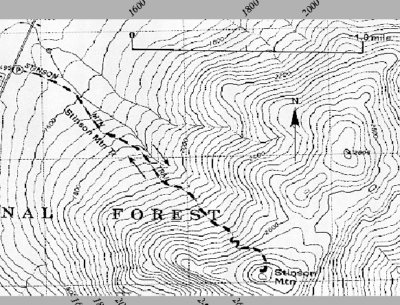
Now let us consider a particular function f of two variables, the altitude function for the region in New Hampshire including Stinson Mountain. We are interested in computing the average and instantaneous rate of change of the altitude function along a path. We will work from a contour map of the region. (Note that the altitude change between adjacent contour lines on the plot is 40 feet and the scale of the map is indicated in the legend.)

(a)

Suppose that P and Q are fixed points on the contour map. Let us consider the line segment from P to Q. How would you compute the average rate of change of the altitude function over this segment? Express your answer in prose and in symbols.

(b)

How would you compute the instantaneous rate of change of the altitude function along this segment at P? Express your answer in prose and symbols.

(c)

What information would you need to carry out the calculation of the instantaneous rate of change in 2(b)? Is it possible to obtain this information from a contour map? Explain. If it is not possible to obtain this information from a contour map, explain how you would approximate the instantaneous rate of change from the contour map.

(d)

Let us focus on the trail on the map leading up the side of Stinson Mountain. Let P be the point where the trail crosses the 1600 ft. contour and let Q be the point where the trail crosses the 1800 ft. contour. The trail is reasonably straight between these two points. Apply your method from 2(a) to calculate the average rate of change of the altitude function on this path from P to Q.

(e)

If possible, use the method you described in 2(b) to calculate the instantaneous rate of change of the altitude function along this path at the point P. If it is not possible, calculate the approximation to the rate of change that you described in 2(c).

3.

We will continue to use the particular point P described in Exercise 2(d). Choose a point Q₀ on the contour plot, different from the original Q and consider the line segment from P to Q₀. As above, it is possible to compute the instantaneous rate of change of the altitude function along the segment from P to Q₀. In general, this instantaneous rate of change will not be the same as the value you computed in Exercise 2(e), thus we should think about how the instantaneous rate of change of the altitude function at P along a line segment depends upon the point Q₀ chosen.

(a)

Suppose Q₀ lies on the line from P through the original point Q. What is the relationship between the instantaneous rate of change of altitude at P along the line segment from P to Q₀ and the instantaneous rate of change of altitude at P along the line segment from P to Q ? Explain your answer.

(b)

Now suppose Q₀ is any point on the contour plot different from P. For which points Q₀ will the instantaneous rate of change of altitude at P along the line segment to Q₀ be positive? Indicate these points on the contour plot and justify your choice.

(c)

For which points Q₀ will the instantaneous rate of change of altitude at P along the line segment to Q₀ be negative? Indicate these points on the contour plot and justify your choice.

(d)

For which points Q₀ will the instantaneous rate of change of altitude at P along the line segment to Q₀ be zero? Indicate these points on the contour plot and justify your choice.

  

Figure: A contour plot of the region near Stinson Mt. in New Hampshire.

startsection section10mm-.5 Discussion 17 Local Linearity of Functions of Two Variables

 

This is a L^ATEXversion of a Maple worksheet. The worksheet is available in the directory /home/stu/courses/math141.

startsection subsection10mm.5 Introduction

In this Maple worksheet we will explore the differentiability of functions of two variables. In particular we would like to investigate the relationship between the existence of the partial derivatives of f at a point and the differentiability of f.