Optimization

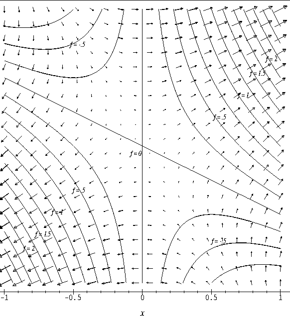
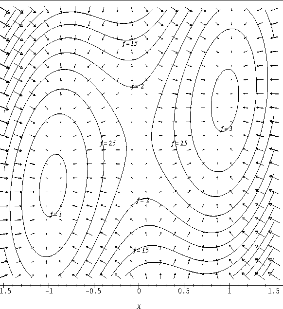
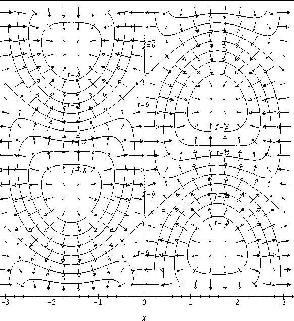
startsection section10mm-.5 Discussion 19 Critical Points

 

In this discussion, we investigate the relative extrema of a function of two variables. In one variable calculus we began our analysis of extreme points by locating the critical points of the function, that is, points where the derivative is zero. We have an analogous definition for functions of two variables.

Definition

A point ${\bf x}_0 = (x_0,y_0)$ is called a critical point of f if

$$\frac{\partial f}{\partial x}({\bf x}_0) = 0\ \ \mbox{and \ \ } \frac{\partial f}{\partial y}({\bf x}_0) = 0.$$

We have already seen in class that we can classify these critical points as relative maxima, relative minima or saddle points by considering the contour plot of f in an open set containing the critical point. In this discussion we will develop another graphical technique for classifying the critical points of f.

Recall that if f is a differentiable function defined on the open set ${\cal D} \subset {\bf R}^2$, the gradient vector of f, $\nabla f({\bf x})$ is defined at every point ${\bf x}\in {\cal D}$. Thus we can define a vector field on ${\cal D}$, called the gradient vector field of f, whose coordinate functions are the first partial derivatives of f. That is,

$$\nabla f({\bf x}) = \left( \frac{\partial f}{\partial x}({\bf x}), \frac{\partial f}{\partial y}({\bf x}) \right),$$

for any ${\bf x}\in {\cal D}$. The critical points of f are then exactly those points which are critical points of the vector field $\nabla f$.

The goal in this discussion is to use a classification of the critical points of the vector field $\nabla f$ to determine a classification of critical points of f.

startsection subsection10mm.5 Exercises

1.

Attached to this discussion you will find plots of the vector field $\nabla f$ displayed on the contour plot of f for three different functions f. On each plot,

(a)

locate the critical points of the vector field,

(b)

sketch several flow lines of the vector field, and

(c)

classify the critical points of the vector field.

2.

Based on the plots of $\nabla f$ and the contours of f that you considered in Exercise 1, and your knowledge of the gradient vector, what is the relationship between the flow lines of f and the contours of f? What happens to the values of f as you move along a flow line?

3.

We determined in our analysis of vector fields that there are four different types of critical points: sinks, sources, saddles and centers. We've seen that the critical points of a function f can be classified as maxima, minima or saddle points. Explain how you would use the classification of critical points of the vector field, $\nabla f$ to classify the critical points of the function f. Based upon the correspondence you have established between the types of critical points of $\nabla f$ and the types of critical points of f, are there any types of critical points for vector fields which you would not expect to find as critical points of gradient vector fields?

  

Figure: Gradient vector field 1.

  

Figure: Gradient vector field 2.

  

Figure: Gradient vector field 3.

startsection section10mm-.5 Discussion 24 Using Maple to Find Critical Points

 

This is a L^ATEXversion of a Maple worksheet. The worksheet is available in the directory /home/stu/courses/math141.

startsection subsection10mm.5 Introduction

In this discussion we would like to use both the graphical and numerical capabilities of Maple to locate and identify critical points of functions of two variables.

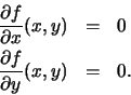
As we have seen in the text, a critical point of a differentiable function f = f(x,y) of two variables is a point for which the gradient vector is equal to zero. That is, (x,y) satsifies:

$$(\frac{\partial f}{\partial x}(x,y), \frac{\partial f}{\partial y}(x,y)) = (0,0).$$

This is equivalent to the following system of equations in two unknowns:

$$\begin{eqnarray*}\frac{\partial f}{\partial x}(x,y)&=&0\\ \frac{\partial f}{\partial y}(x,y) &=&0. \end{eqnarray*}$$

In Discussion of Chapter 3, we saw how to solve systems of two equations in two variables numerically by the Newton-Raphson method and we used a procedure, newrap, to carry out the calculations. In this discussion we will use the built-in Maple numerical equation solving routine, fsolve, which utilizes a modified form of the Newton-Raphson method. Unlike newrap, fsolve does not give the user control of the number of iterates used to produce the solution. In the following example, we will see how to use fsolve and the built-in Maple plotting commands.

startsection subsection10mm.5 An Example

Let us use the Maple plotting commands and fsolve to find and identify the critical points of the function.

    f:=(x,y)->  y^3 - 2*y -5 - 3*x^2;

In order to make a preliminary guess about the number of critical points, let us examine a contour plot of f. Note that we are confining our attention to the rectangle $[-2,2]\times [-2,2]$, so that initially we will only find critical points in this region. It is possible-though it is not the case for this function-that the region we choose to graph might not contain all the critical points of a function. Thus we might have to consider the behavior on different regions in order to find all the critical points.

    contourplot(f(x,y),x=-2..2,y=-2..2);

Based upon the plot, we expect that f has a critical point located at approximately (0,-.8) that is a maximum or minimum and a critical point located at approximately (0, .8). In order to obtain a more accurate approximation, we can employ fsolve. The fsolve command will solve a system of equations for several variables in a specific region. A convenient way to do this is first define the set of equations and then define the set of variables. Notice that we are using the operator D to compute the partial derivatives of f. For example, D[1](f) is the partial derivative of f with respect to the first variable in the definition of f, which is xin this case.

    eqns:={D[1](f)(x,y) = 0, D[2](f)(x,y)=0};
    vars:={x,y};

The following use of fsolve does not specify a region. Let us see what happens:

    fsolve(eqns,vars);

This returns a single critical point that is approximately located at (0,-.8165). (Note that the full value to 10 decimal places is still only an approximation to a solution.) Apparently, this is the critical point that we located at (0,-.8). To find the other critical point, let us specify a domain.

    fsolve(eqns,vars,y=0..1);

This yields the other critical point which is approximately located at (0, .8165). Note that if the region is left unspecified, the numerical values generated by fsolve may fail to converge. To remedy this problem, you must specify a region.

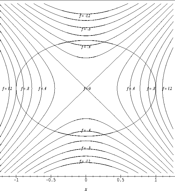
To identify the type of these critical points, we might use contourplot, but display more contours and focus our attention on region containing a critical point:

    contourplot(f(x,y),x=-.5 .. .5,y=.5.. 1.5,contours=25);

We see that the contours appear to form a family of hyperbolas, which indicates that the critical point is a saddle. We might also plot the graph of the function on the same region.

    plot3d(f(x,y),x=-.5.. .5, y= .5 .. 1.5,axes = BOXED,
                 style=PATCHCONTOUR,view=-6.4..-5);

Notice in the preceding plot3d command we specified several options. We chose the axes to appear as the frame of a box; we chose the plot to be shaded and to display horizontal slices, and we restricted the vertical portion of the plot to the interval [-6.4,-5]. This last option is particularly useful since it can eliminate portions of the graph whose z-values are not close to the value at the critical point.

In a similar manner we could examine the behavior of f in a region containing the other critical point. We would find that it is a local maximum.

In this case, it is apparent from the equations that f has no other critical points, so we are done.

startsection subsection10mm.5 Exercises

For each of the following functions, use Maple to locate and identify all the critical points. As above, you should use the contour plot to determine the approximate location of the critical points and then use fsolve to locate them more precisely. If you find that a critical point is difficult to locate or identify, explain why the behavior of the function made it difficult to locate.

Before starting the exercises be sure to load the plots package:

    with(plots):

When working with a new function, enter the following definitions after defining the function and before using fsolve.

    eqns:={D[1](f)(x,y) = 0, D[2](f)(x,y)=0}:
    vars:={x,y}:

When working with a new function, enter the following definitions.

1.

f:=(x,y)-> -x^2*(x^2 - 4) + y^4 + x^2 + y^2:

2.

This function is expressed in terms of the hyperbolic secant functions, sech, which is defined by

$$\mbox{sech}(u) = 2/(e^u + e^{-u}).$$

f:=(x,y)-> sech((x+.5)^2 + y^2) + 2*sech((x-1)^2 + (y-2)^2):

3.

f:=(x,y)->1/(1 + x^2 + (y-1)^2) - 2/(1 +(x-1)^2 + (y-x)^2);

startsection section10mm-.5 Discussion 25 The Second Derivative Test

 

In this discussion we will apply the second derivative test to two functions. First, let us review the hypothesis of the second derivative test. We must have that f is a twice differentiable function of two variables and that (x₀,y₀) is a critical point of f, that is, $\nabla f(x_0,y_0) = (0,0)$. Let

$$A = \frac{\partial^2 f}{\partial x^2}(x_0,y_0), \ \ B =\frac... ..., \mbox{ and } C = \frac{\partial^2 f}{\partial y^2}(x_0,y_0),$$

If $AC -B^2 \neq 0$, we say that the critical point is non-degenerate. In this case, the second derivative test will tell us the type of the critical point. If AC-B² = 0 we call the critical point degenerate. The test does not apply in this case and we must use other means to identify the type of the critical point. In particular, we might use graphical techniques or we might directly analyze the symbolic expression for f.

startsection subsection10mm.5 Exercises For each of the following functions

(i) Compute the partial derivatives $\frac{\partial f}{\partial x}(x,y)$ and $\frac{\partial f}{\partial y}(x,y)$.
(ii) Find the critical points of f.
(iii) Compute the second partial derivatives of f.
(iv) Use the second derivative test to classify the non-degenerate critical points of f.
(v) If there are any degenerate critical points, use another method to determine if these critical points are local maxima, local minima or saddle points.

1.

f(x,y) = x³ - 6xy + y³.

2.

$f(x,y) = x^4 + \frac{1}{2}y^4 -4xy^2 +2x^2 +2y^2 +1.$

startsection section10mm-.5 Discussion 26 Constrained Optimization

 

We have so far developed geometric and symbolic methods to locate and classify relative extrema of a differentiable function f on an open set in ${\bf R}^2$. In this discussion, we want to extend these techniques so that we can locate extrema on a closed set ${\cal S}$ consisting of an open set ${\cal O}$ and its boundary curve ${\cal B}$. The extrema for f on ${\cal S}$ must occur at either the relative extrema of f on ${\cal O}$ or at the relative extrema of f on ${\cal B}$. Since we already have techniques for finding relative extrema on ${\cal O}$, we need only develop a technique for locating relative extrema on ${\cal B}$. Here we will consider the case where ${\cal B}$, the boundary of ${\cal S}$, is a set of points satisfying an equation of the form g(x,y) = c, where g is a differentiable function. We will call a condition of this type a constraint and speak of optimizing fsubject to a constraint.

In this discussion we will approach the problem of locating the extrema of f subject to the constraint g(x,y) = c by considering the relationship between the level sets of f and the curve g(x,y) = c. Our aim is to give a graphical characterization of the extreme points of f on this boundary curve, and to use this to produce a symbolic characterization that will lead to a symbolic solution of the problem.

startsection subsection10mm.5 Exercises

1.

Attached to this discussion are plots for three constrained optimization problems. Each plot consists of the contours of a differentiable function f and the boundary curve g(x,y) =c.

(a)

For each plot, use the values assigned to the contours to locate the maximum and minimum values of f on the boundary curve.

(b)

What is the relationship between the contour curve of f and the boundary curve at the extreme points?

(c)

We have seen that the vector field $\nabla f$ can provide information for analyzing extreme values of f. For each plot, sketch $\nabla f$ on the contour plot. What is the relationship between $\nabla f$ and the boundary curve at the extreme points of f on the boundary curve?

(d)

The boundary curve g(x,y) = c is a level set for the differentiable function g. What does this imply about the relationship between $\nabla g$ and the boundary curve?

(e)

What is the relationship between $\nabla f$ and $\nabla g$ at the extreme points of f on the boundary curve?

2.

(a)

Use your graphical characterization from Exercise 1 to produce a symbolic characterization of the extreme points of f subject to the constraint g(x,y) = c.

(b)

How would you use this symbolic characterization to algebraically solve for the extreme points of f subject to the constraint g(x,y) = c.

3.

Consider the three plots again.

(a)

Are there other points on the boundary curve which would satisfy the graphical conditions you summarized in Exercise 1? Locate these points.

(b)

What is the behavior of f on the boundary curve at these points?

  

Figure: Constrained optimization problem 1.

  

Figure: Constrained optimization problem 2.

  

Figure: Constrained optimization problem 3.

startsection section10mm-.5 Discussion 27 Lagrange Multipliers

 

In this discussion we will work through examples of finding the extreme values of a function on a closed set ${\cal S} = {\cal O} \cup {\cal B}$. Let f be a differentiable function defined on an open set containing ${\cal S}$. We will locate the critical points of f on ${\cal O}$, the interior of ${\cal S}$ by solving the equation $\nabla f ({\bf x}) = {\bf0}$. We will then use the method of Lagrange multipliers to locate the extreme values of f on the boundary ${\cal B}$. Let us recall the statement of the method.

Assume ${\cal B}$ is described by the equation g(x,y) = c, where g is a differentiable function and $\nabla g \neq {\bf0}$ on ${\cal B}$. Then the extreme values of f on ${\cal B}$ occur at solutions to the system of equations

$$\frac{\partial f}{\partial x}(x,y) \lambda \frac{\partial g}{\partial x}(x,y)$$ =

$$\frac{\partial f}{\partial y}(x,y) \lambda \frac{\partial g}{\partial y}(x,y)$$ =

g(x,y) = c.

Recall that not all the points that are critical points in ${\cal O}$or solve the Lagrange system of equations on ${\cal B}$ are absolute minima and maxima. In order to determine which of the points are absolute minima and maxima, it is necessary to substitute the x and y solution values into the function f and choose the points that give the largest value of f and the points that give the smallest value of f.

startsection subsection10mm.5 Exercises

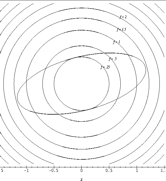
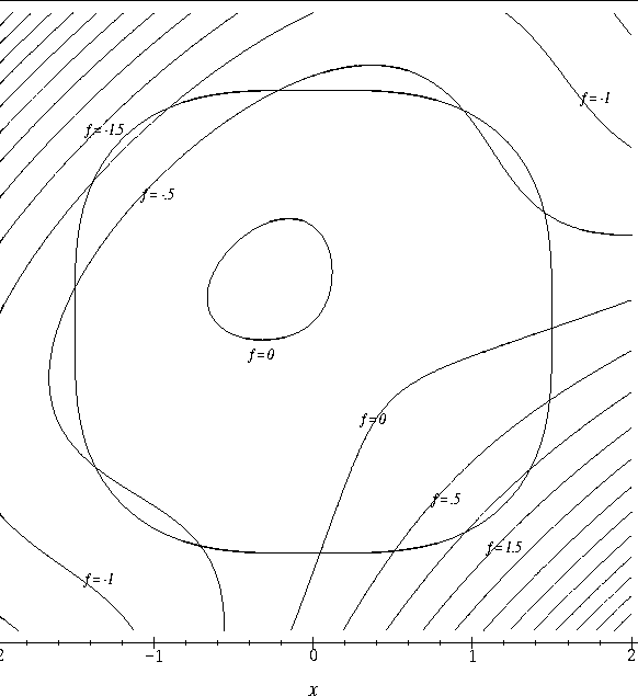
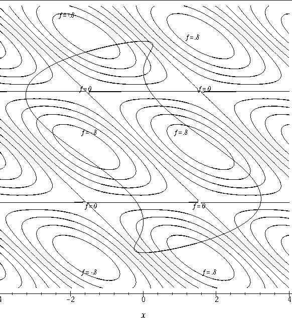
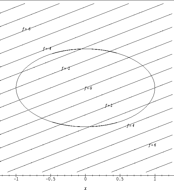
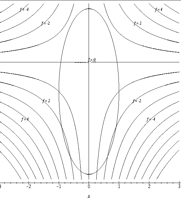
Attached to the discussion sheet are plots for the following three constrained optimization problems. Each plot consists of the contours of a function f and the curve which is the boundary of ${\cal S}$. For each of these problems, locate the critical points of f on ${\cal O}$, the interior of the closed set ${\cal S}$, on the plot and then solve the equation $\nabla f ({\bf x}) = {\bf0}$ to determine these points symbolically. Then use the plot to locate the relative and absolute extreme points of f on the boundary curve and write out and solve the Lagrange multiplier system of equations in order to find the coordinates of the extreme points of f subject to the constraint. Keep in mind that while you cannot find exact values for the coordinates of the extreme points from the contour plot, you can use the plot to determine the number and type of the extreme points.

1.

Find the extreme values of f(x,y) = 2x - 5y on the closed set

$${\cal S} = \{(x,y) \: : \: x^{2} + 3y^{2} \leq 1.\}$$

(See Figure .)

2.

Find the extreme values of f(x,y) = x² - y² on the closed set

$${\cal S} = \{ (x,y) \: : \: x^{2} + 2y^{2} \leq 1.\}$$

(See Figure .)

3.

Find the extreme values of f(x,y) = xy -x on the closed set

$${\cal S} = \{(x,y) \::\: x^{2} + y^{2}/4 \leq 2.\}$$

(See Figure .)

  

Figure: A contour plot for f(x,y)=2x - 5y showing the contraint curve g(x,y) = x² + 3y² = 1.

  

Figure: A contour plot for f(x,y) = x² - y² showing the constraint curve g(x,y) = x² + 2y² = 1.

  

Figure: A contour plot for f(x,y) = xy-x showing the constraint curve g(x,y) = x² + y²/4 = 2.