MATH 392 -- Seminar in Computational Commutative Algebra
October 16, 2006
More on the geometry of envelopes of families of curves
Consider the family of normal lines to the parabola ![]()
(A normal line is a line passing through a point on the parabola,
perpendicular to the tangent line of the parabola at that point.)
Since ![]() at a point
at a point ![]() on the parabola, the
on the parabola, the
equation of the normal line will be ![]()
Clearing denominators we have
![]()
is the function of three variables defining the family of normal
lines.
| > |
| > |
![]()
| > |
There are several ways to visualize this, either by using ![]() as an
as an
"animation variable" as we saw in problem II on the Midterm Problem
Set, or alternatively by considering the variety ![]()
in ![]() .
.
In the Midterm Problem Set, we introduced the envelope of the
family by saying we wanted to produce a curve that was
tangent to the curves in the family. This is useful as an
intuitive way to visualize the envelope, but it is somewhat
imprecise for several reasons:
1. The curves in a family can intersect the envelope at some
points where they are tangent to the envelope, but at
other points too, where they are not tangent to the envelope.
2. The envelope curve itself can have singular points such
as cusp points, where it is not clear what saying
another curve is tangent to the envelope should mean.
So a somewhat better way to think of the equations
![]()
![]()
which appear in the definition of the envelope is that they define
a subset (usually a curve) on the surface
![]()
in ![]() called the "apparent contour" -- the set of points where
called the "apparent contour" -- the set of points where
the tangent plane to V is vertical. When we eliminate the variable t
to get the envelope equation, we are finding the projection of
the apparent contour into the xy - plane.
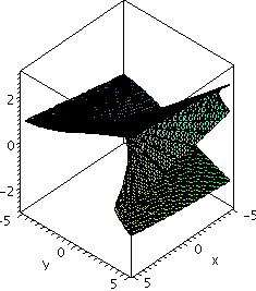
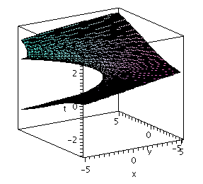
Here are two implicit plots of the surface V for the family
of normal lines to the parabola, from two different points of view,
showing where the envelope and the apparent contour of the surface
come from. Here is what to look for in these:
* In the first one, look for a "lower fold" of the surface giving
points on the apparent contour with ![]()
* In the second, look for an "upper fold" giving points on the apparent
contour with ![]()
| > |
| > |
| > |
| > |
We can find the equation of the apparent countour or envelope of the family
by using a lex Grobner basis (![]() to eliminate
to eliminate ![]() between the equations
between the equations ![]()
![]()
and ![]() as discussed in the Midterm Problem Set (and Chapter 3, section 4
as discussed in the Midterm Problem Set (and Chapter 3, section 4
in the text).
| > |
![]()
![]()
| > |
![]()
The first element of the Grobner basis defines the envelope (projection of the
apparent contour):
| > |
![]()
The other elements of the Grobner basis look like this:
| > |
![]()
![]()
| > |
![]()
Here is an animated display showing
* the lines in the family of normal lines (in blue)
* the envelope (in red)
* the parabola (in black)
| > |
| > |
| > |
| > |
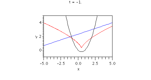
Note that in this case the envelope curve does apparently have a cusp
point. We can find the coordinates by solving the equations
![]() point is on the envelope)
point is on the envelope)
![]() (tangent line to the envelope not well-defined)
(tangent line to the envelope not well-defined)
![]()
| > |
![]()
| > |
There is actually just one point in the variety defined here: ![]()
which is where the cusp point is located. Note that this point is also
where "special behavior" of the Grobner basis B occurs -- It's exactly
that point where the Grobner basis polynomials B[2] and B[3] become
0 for all t.