MATH 376 -- Probability and Statistics II 

Type II Error Probabilities for a large-sample lower-tail Z-test 

March 25, 2010 

We consider testing for value of a proportion.  Say the null  

hypothesis is :  p = .3  and the alternative hypothesis is 

:  p < .3.  We will assume  n  is always large enough 

so that our general discussions of the large-sample tests applies.  

The test statistic is   z =  and the rejection region for 

an -level test is  RR = { z < - z_.05 } = { z < -1.645 }  or  {Y/n < .3 - 1.645 }. 

Set-up: 

>	sigma[1]:=n->sqrt((.3)*(.7)/n);

 

(1)

 

The normal pdf under the assumption that    is true: 

>	f[1]:=n->1/sqrt(2*Pi*sigma[1](n)^2)*exp(-(y-.3)^2/(2*sigma[1](n)^2));

 

(2)

 

But now suppose that the actual value of  p  is  .24.  We ask:  How likely are 

we to make a Type II error with the = .05-level rejection region given above? 

Here's the normal pdf that approximates the distribution with  p = .24: 

>	sigma[2]:=n->sqrt((.24)*(.76)/n);

 

(3)

 

>	f[2]:=n->1/sqrt(2*Pi*sigma[2](n)^2)*exp(-(y-.24)^2/(2*sigma[2](n)^2));

 

(4)

 

>	RR:=n->.3-1.645*sigma[1](n);

 

(5)

 

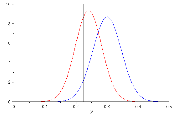
The following plot shows the normal densities for the sampling distribution  

of Y/100: 

   blue plot (shorter normal curve) = if  is true 

   red plot (taller normal curve) = if  is false and actual  p = .24 

The vertical black line is plotted at the value .2246 (the upper edge of the RR taking  

n = 100.) 

>

RR(100);

 

(6)

 

>	Dists:=plot([f[1](100),f[2](100)],y=0..0.5,color=[blue,red]):

 

>	RRPlot:=plot([RR(100),t,t=0..10],color=black):

 

>	with(plots):

 

>	display(Dists,RRPlot);

 

The area under the shorter normal curve to the left of the vertical line is the probability 

of a Type I error: 

>	evalf(Int(f[1](100),y=-infinity..RR(100)));

 

(7)

 

This checks with the desired value   = .05 The area under the taller normal curve to the  

right of the vertical line is the probability of a Type II error (always assuming  p = .24): 

>	evalf(Int(f[2](100),y=RR(100)..infinity));

 

(8)

 

This is certainly unacceptably large!  What can we do to decrease it?   

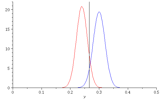
The answer is:  Increase the sample size(!) Increasing n decreases the variances of both  

distributions (so the pdf's get taller and skinnier), and moves the cut-off for the RR for the  

.05-level test farther to the right.  For instance the picture for n = 500 is: 

>

RR(500);

 

(9)

 

>	Dists:=plot([f[1](500),f[2](500)],y=0..0.5,color=[blue,red]):

 

>	RRPlot:=plot([RR(500),t,t=0..22],color=black):

 

>	display(Dists,RRPlot);

 

>

 

(10)

 

>	evalf(Int(f[2](500),y=RR(500)..infinity));

 

(11)

 

So the Type II error probability    has been reduced to .084 by increasing  n  to 500, 

while = .05 still.  In class we showed that  can be reduced to any given value 

by taking n sufficiently large.