MATH 376 -- Probability and Statistics 2 

April 12, 2010 

First Least Squares Regression Example 

>	with(Statistics):

 

For computation of the estimators for the coefficients in the model 

  Y =  

We enter the lists of x  and  y  coordinates of the data points separately: 

>	XList:=[0.,1,2,3,4,5,6,7];

 

(1)

 

>	YList:=[34.3,33.5,35.9,39.3,44.8,48.8,55.7,62.9];

 

(2)

 

Means: 

>	Xbar:=Mean(XList);

 

(3)

 

>	Ybar:=Mean(YList);

 

(4)

 

Organizing the computation as we described in class: 

>	SXY:=add((XList[i]-Xbar)*(YList[i]-Ybar),i=1..8);

 

(5)

 

>	SXX:=add((XList[i]-Xbar)*(XList[i]-Xbar),i=1..8);

 

(6)

 

>	hatbeta[1]:=SXY/SXX;

 

(7)

 

>	hatbeta[0]:=Ybar-hatbeta[1]*Xbar;

 

(8)

 

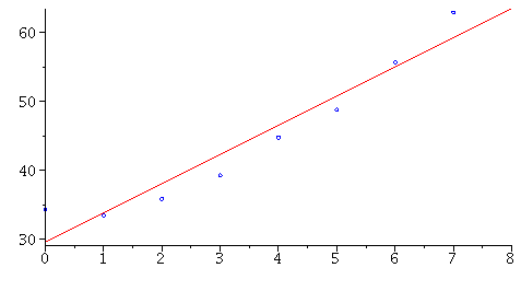
Plot the data points together with the line determined by the least-squares estimators 

for  and  

>	with(plots):

 

>	Pts:=[seq([XList[i],YList[i]],i=1..8)];

 

(9)

 

>	PP:=plot(Pts,style=point,color=blue,symbol=circle):

 

>	LP:=plot(hatbeta[0]+hatbeta[1]*x,x=0..8):

 

>	display(PP,LP);

 

>

 

This indicates an OK (but not ideal) "fit" with the linear model.   

Other functional forms might also be considered, since  

it seems that the y's are consistently low in the middle of the range  

of x's and consistently high on the ends.  A truly good fit with  

a model of our form will have points ``randomly'' high and low 

with respect to the regression line.