PS 8 Solutions
11.8
| > |
read "/home/fac/little/public_html/ProbStat0910/MSP.map"; |
| Warning, the use of _seed is deprecated. Please consider using one of the alternatives listed on the _seed help page. |
 |
(1) |
| > |
XList:=[39.0,37.5,22.2,17.5,.64,.45,2.62,2.36,32.0,.77]; |
![[39.0, 37.5, 22.2, 17.5, .64, .45, 2.62, 2.36, 32.0, .77]](images/PS2PS8Sols_2.gif) |
(2) |
| > |
YList:=[23.0,22.3,9.4,9.7,.15,.28,.75,.51,28.,.39]; |
![[23.0, 22.3, 9.4, 9.7, .15, .28, .75, .51, 28., .39]](images/PS2PS8Sols_3.gif) |
(3) |
 |
(4) |
 |
(5) |
| > |
Sxx:=add((XList[i]-Xbar)^2,i=1..nops(XList)); |
 |
(6) |
| > |
Sxy:=add((XList[i]-Xbar)*(YList[i]-Ybar),i=1..nops(XList)); |
 |
(7) |
| > |
Syy:=add((YList[i]-Ybar)^2,i=1..nops(YList)); |
 |
(8) |
 |
(9) |
| > |
beta[0]:=Ybar-beta[1]*Xbar; |
 |
(10) |
| > |
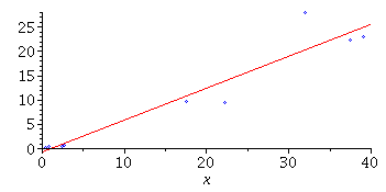
PP:=plot([seq([XList[i],YList[i]],i=1..nops(XList))],style=point,symbol=diamond,color=blue): |
| > |
LP:=plot(beta[0]+beta[1]*x,x=0..40,color=red): |
Estimate of value for x = 12:
 |
(11) |
11.12
a)
| > |
XList:=[0.0,4,14,32,52]; |
![[0., 4, 14, 32, 52]](images/PS2PS8Sols_13.gif) |
(12) |
| > |
YList:=[19.8,16.5,12.8,8.1,7.5]; |
![[19.8, 16.5, 12.8, 8.1, 7.5]](images/PS2PS8Sols_14.gif) |
(13) |
 |
(14) |
 |
(15) |
| > |
Sxx:=add((XList[i]-Xbar)^2,i=1..nops(XList)); |
 |
(16) |
| > |
Sxy:=add((XList[i]-Xbar)*(YList[i]-Ybar),i=1..nops(XList)); |
 |
(17) |
| > |
Syy:=add((YList[i]-Ybar)^2,i=1..nops(YList)); |
 |
(18) |
 |
(19) |
| > |
beta[0]:=Ybar-beta[1]*Xbar; |
 |
(20) |
b)
| > |
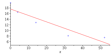
PP:=plot([seq([XList[i],YList[i]],i=1..nops(XList))],style=point,symbol=diamond,color=blue): |
| > |
LP:=plot(beta[0]+beta[1]*x,x=0..55,color=red): |
c) Estimate for x = 20:
 |
(21) |
11.13
| > |
XList:=[7.23,8.53,9.82,10.26,8.96,12.27,10.28,4.45,1.78,4.0,3.3,4.3,0.8,0.5]; |
![[7.23, 8.53, 9.82, 10.26, 8.96, 12.27, 10.28, 4.45, 1.78, 4.0, 3.3, 4.3, .8, .5]](images/PS2PS8Sols_24.gif) |
(22) |
| > |
YList:=[190,160,134,129,172,197,167,239,542,372,245,376,454,410]; |
![[190, 160, 134, 129, 172, 197, 167, 239, 542, 372, 245, 376, 454, 410]](images/PS2PS8Sols_25.gif) |
(23) |
| > |
Xbar:=add(XList[i],i=1..nops(XList))/nops(XList); |
 |
(24) |
| > |
Ybar:=add(evalf(YList[i]),i=1..nops(YList))/nops(YList); |
 |
(25) |
| > |
Sxx:=add((XList[i]-Xbar)^2,i=1..nops(XList)); |
 |
(26) |
| > |
Sxy:=add((XList[i]-Xbar)*(YList[i]-Ybar),i=1..nops(XList)); |
 |
(27) |
| > |
Syy:=add((YList[i]-Ybar)^2,i=1..nops(YList)); |
 |
(28) |
 |
(29) |
| > |
beta[0]:=Ybar-beta[1]*Xbar; |
 |
(30) |
So the line is: y = 
 x
x
b) The plot of the data points with the regression line:
| > |
PP:=plot([seq([XList[i],YList[i]],i=1..nops(XList))],style=point,symbol=diamond,color=blue): |
| > |
LP:=plot(beta[0]+beta[1]*x,x=0..14,color=red): |
11.24
We must test the null hypothesis  :
:  against the alternative
 |
(31) |
| > |
S:=sqrt(SSE/(nops(XList)-2)); |
 |
(32) |
| > |
t:=beta[1]/(S*sqrt(1/Sxx)); |
 |
(33) |
 |
(34) |
The p-value of the test is < 2(.005) since  so we reject the
null hypothesis if  . A more accurate estimate of the p-value is:
| > |
p:=2*(1-TCDF(12,5.775)); |
 |
(35) |
11.26
a)
| > |
XList:=[29.4,39.2,49.0,58.8,68.6,78.4]; |
![[29.4, 39.2, 49.0, 58.8, 68.6, 78.4]](images/PS2PS8Sols_46.gif) |
(36) |
| > |
YList:=[4.25,5.25,6.5,7.85,8.75,10.0]; |
![[4.25, 5.25, 6.5, 7.85, 8.75, 10.0]](images/PS2PS8Sols_47.gif) |
(37) |
| > |
Xbar:=add(XList[i],i=1..nops(XList))/nops(XList); |
 |
(38) |
| > |
Ybar:=add(evalf(YList[i]),i=1..nops(YList))/nops(YList); |
 |
(39) |
| > |
Sxx:=add((XList[i]-Xbar)^2,i=1..nops(XList)); |
 |
(40) |
| > |
Sxy:=add((XList[i]-Xbar)*(YList[i]-Ybar),i=1..nops(XList)); |
 |
(41) |
| > |
Syy:=add((YList[i]-Ybar)^2,i=1..nops(YList)); |
 |
(42) |
 |
(43) |
| > |
beta[0]:=Ybar-beta[1]*Xbar; |
 |
(44) |
b)
| > |
S:=sqrt((Syy-beta[1]*Sxy)/4); |
 |
(45) |
 |
(46) |
From table in text, 
| > |
beta[1]-2.776*S*sqrt(c11),beta[1]+2.776*S*sqrt(c11); |
 |
(47) |
c)
| > |
c00:=add(XList[i]^2,i=1..6)/(6*Sxx); |
 |
(48) |
| > |
t:=beta[0]/(S*sqrt(c00)); |
 |
(49) |
 |
(50) |
p = attained sig. level is = is between 2(.01) = .02 and 2(.005) = .01
since t_(.01)(4) = 3.747 and t_(.005)(4) = 4.604. At  ,
,
we would reject the null hypothesis and conclude  .
.
(11.27 on other sheets)
11.69
a)
| > |
XList:=[-7.,-5.,-3.,-1.,1.,3.,5.,7.]; |
![[-7., -5., -3., -1., 1., 3., 5., 7.]](images/PS2PS8Sols_64.gif) |
(51) |
| > |
YList:=[18.5,22.6,27.2,31.2,33.0,44.9,49.4,35.0]; |
![[18.5, 22.6, 27.2, 31.2, 33.0, 44.9, 49.4, 35.0]](images/PS2PS8Sols_65.gif) |
(52) |
 |
(53) |
 |
(54) |
| > |
Sxx:=add((XList[i]-Xbar)^2,i=1..nops(XList)); |
 |
(55) |
| > |
Sxy:=add((XList[i]-Xbar)*(YList[i]-Ybar),i=1..nops(XList)); |
 |
(56) |
| > |
Syy:=add((YList[i]-Ybar)^2,i=1..nops(YList)); |
 |
(57) |
 |
(58) |
| > |
beta[0]:=Ybar-beta[1]*Xbar; |
 |
(59) |
Using matrix formuation. The model Y = 
| > |
X:=transpose(stackmatrix([seq(1,i=1..nops(XList))],[XList])); |
 |
(60) |
| > |
M:=multiply(transpose(X),X); |
![array( 1 .. 2, 1 .. 2, [( 2, 2 ) = 168., ( 2, 1 ) = 0., ( 1, 2 ) = 0., ( 1, 1 ) = 8 ] )](images/PS2PS8Sols_75.gif) |
(61) |
| > |
linsolve(M,multiply(transpose(X),YList)); |
![array( 1 .. 2, [( 1 ) = 32.72500000, ( 2 ) = 1.811904762 ] )](images/PS2PS8Sols_76.gif) |
(62) |
The model Y = 
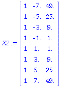
| > |
X2:=transpose(stackmatrix([seq(1,i=1..nops(XList))],[XList],[seq(XList[i]^2,i=1..nops(XList))])); |
 |
(63) |
| > |
M2:=multiply(transpose(X2),X2); |
![array( 1 .. 3, 1 .. 3, [( 2, 2 ) = 168., ( 2, 1 ) = 0., ( 1, 2 ) = 0., ( 1, 1 ) = 8, ( 2, 3 ) = 0., ( 1, 3 ) = 168., ( 3, 1 ) = 168., ( 3, 3 ) = 6216., ( 3, 2 ) = 0. ] )](images/PS2PS8Sols_79.gif) |
(64) |
| > |
linsolve(M2,multiply(transpose(X2),YList)); |
![array( 1 .. 3, [( 1 ) = 35.56249999, ( 2 ) = 1.811904762, ( 3 ) = -.1351190473 ] )](images/PS2PS8Sols_80.gif) |
(65) |
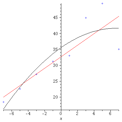
| > |
PP:=plot([seq([XList[i],YList[i]],i=1..nops(XList))],style=point,symbol=diamond,color=blue): |
| > |
LP:=plot(32.725+1.812*x,x=-7..7,color=red): |
| > |
 |
In this case , it is more or less clear from the graphs that the point [7,35] from
the year 2003 is the ``culprit'' here. If we excluded that point, the model Y = ![`+`(beta[0], `*`(beta[1], `*`(x)), epsilon)](images/PS2PS8Sols_83.gif) would fit very well and the quadratic model Y =
would fit very well and the quadratic model Y = ![`+`(beta[0], `*`(beta[1], `*`(x)), `*`(beta[2], `*`(`^`(x, 2))), epsilon)](images/PS2PS8Sols_84.gif) would not be
would not be
much of an improvement. With that point, neither model is all that good for  (!)
(!)
![]()
![]() x
x 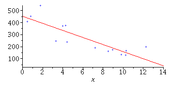
![]() :
: ![]() against the alternative
against the alternative ![]()
![]() so we reject the
so we reject the ![]() . A more accurate estimate of the p-value is:
. A more accurate estimate of the p-value is: ![]()
![]() ,
, ![]() .
. ![]()

![]()

![array( 1 .. 3, 1 .. 3, [( 2, 2 ) = 168., ( 2, 1 ) = 0., ( 1, 2 ) = 0., ( 1, 1 ) = 8, ( 2, 3 ) = 0., ( 1, 3 ) = 168., ( 3, 1 ) = 168., ( 3, 3 ) = 6216., ( 3, 2 ) = 0. ] )](images/PS2PS8Sols_79.gif)
![]() would fit very well and the quadratic model Y =
would fit very well and the quadratic model Y = ![]() would not be
would not be ![]() (!)
(!)