MATH 376 -- Probability and Statistics II
How can we tell if sampled data are coming from a normal population? 

February 25, 2010 

In deriving the small-sample formulas for confidence intervals for 

population means and differences of population means, recall that 

we had to make some rather restrictive additional hypotheses in  

order to apply the facts we know about  t-distributions: 

   *  we need to assume that the samples are drawn from  

      normal populations 

   *  for the difference of means case, we need to assume  

      the two population variances are the same. 

We have seen how to derive some evidence about whether the  

equality of population variances is reasonable, via our confidence 

intervals for   (derived using the F-distribution).   

But this still leaves some questions:   

    1)  Can we test whether it is reasonable to assume the samples 

         are coming from a normal population? 

    2)  How much of a difference does it make if they are not? 

The answer to the second question is basically that it can make 

quite a bit of difference depending on how much the distribution 

deviates from normality.   The distribution of     

can be very different from a t-distribution if the underlying distribution  

is not normal.  Trying to use the formulas we have derived in a case like  

that can yield misleading and/or meaningless results! 

Thus, it becomes important to know that there are ways--some more 

intuitive, some more precise--to get some indication whether it is 

reasonable to make the assumption that a collection of sampled data
has been drawn from a normal population.

The first way we will discuss is a graphical method called the 

Normal Probability Plot.  The idea here is to compare the distribution 

of the sampled data values with the distribution we would expect 

from a normal population in a particular way -- we order the 

sample and compare those ordered values to the  

``normal scores'' --  the expected values of the order statistics for
a sample of the same size drawn from a normal population.     Here
are the necessary calculations.  

The standard normal pdf  and  cdf  first: 

(1)

 

(2)

 

The following computes the expected values for the order statistics
of a sample of size  n  from a standard normal population, using our 

formulas for the  pdfs  of the order statistics: 

(3)

 

(4)

 

Let's apply this to the following collection of 12 net incomes from
a random sample of tax returns: 

(5)

 

 

Warning, the use of _seed is deprecated.  Please consider using one of the alternatives listed on the _seed help page.
	(6)

 

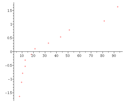
The normal probability plot is just the scatter plot of the points
with the income as x  and the corresponding normal score as y: 

What are we looking for??   Well, if the data are coming from a normal
population, then we would expect the scatter plot to be  nearly a straight line.
Some ``random up and down variation'' from that line would also be expected
because of chance errors coming from the sampling process.

In this example, though, notice that there is an apparent systematic  curvature 

in the scatter plot.   If you see this kind of pattern, it is a strong indication
that assuming normality of the underlying population is probably not justified!!
 

For now, we will leave this discussion at this somewhat intuitive level.  We will 

return to these questions later on, in our discussion of regression (finding a 

line that ``best fits a collection of data'')  and the correlation coefficient that 

we discussed briefly last semester in connection with covariances.   

For your general ``statistical literacy,'' it is also important to be aware that 

there are a number of other much more sophisticated statistical normality 

tests that are commonly used to get information in this situation.   Maple has
one very good one (called the Shapiro-Wilk W Test) as part of its Statistics
package.
 

 

Shapiro and Wilk's W-Test for Normality --------------------------------------- Null Hypothesis: Sample drawn from a population that follows a normal distribution Alt. Hypothesis: Sample drawn from population that does not follow a normal distribution Sample size:             12 Computed statistic:      0.817741 Computed pvalue:         0.0131943 Result: [Rejected] There exists statistical evidence against the null hypothesis

 

We will discuss some of the language involved here -- :"null hypothesis, alternative hypothesis, 

p-value, etc."  after Spring Break.  For now, let us just close by interpreting the results here --  

what this is saying is that there is actually pretty strong evidence to reject the assumption that 

these samples were coming from a normal population!