MATH 376 -- Probability and Statistics 2 

Multiple Regression and Hypothesis testing  

April 26, 2010 

We have two strains of bacteria and want to compare their growth rates.  If we do  

simple regression with each data set as follows: 

>

restart;

 

>	with(Statistics):

 

(1)

 

>	times:=[-2,-1,0,1,2];

 

(2)

 

>	A:=[8.0,9.0,9.1,10.2,10.4];

 

(3)

 

>	B:=[10.0,10.3,12.2,12.6,13.9];

 

(4)

 

>	Tbar:=Mean(times);

 

(5)

 

>	Abar:=Mean(A);

 

(6)

 

>	Bbar:=Mean(B);

 

(7)

 

>	SXYA:=add((times[i]-Tbar)*(A[i]-Abar),i=1..5);

 

(8)

 

>	SXXA:=add((times[i]-Tbar)^2,i=1..5);

 

(9)

 

>	Ahatbeta[1]:=SXYA/SXXA;

 

(10)

 

>	Ahatbeta[0]:=Abar-Ahatbeta[1]*Tbar;

 

(11)

 

>	SXYB:=add((times[i]-Tbar)*(B[i]-Bbar),i=1..5);

 

(12)

 

>	SXXB:=SXXA;

 

(13)

 

>	Bhatbeta[1]:=SXYB/SXXB;

 

(14)

 

>	Bhatbeta[0]:=Bbar-Bhatbeta[1]*Tbar;

 

(15)

 

>	APoints:=[seq([times[i],A[i]],i=1..5)];

 

(16)

 

>	BPoints:=[seq([times[i],B[i]],i=1..5)];

 

(17)

 

>	with(plots):

 

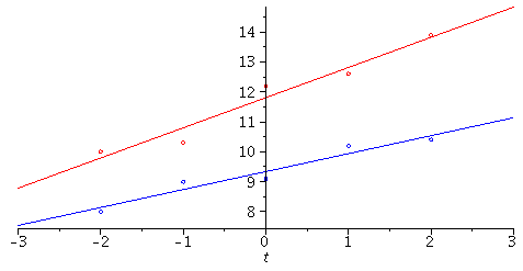
>	AP:=plot(APoints,style=point,symbol=circle,color=blue):

 

>	BP:=plot(BPoints,style=point,symbol=circle,color=red):

 

>	AL:=plot(Ahatbeta[0]+Ahatbeta[1]*t,t=-3..3,color=blue):

 

>	BL:=plot(Bhatbeta[0]+Bhatbeta[1]*t,t=-3..3,color=red):

 

>	display(AP,BP,AL,BL);

 

Note:  From this plot, it seems that the lines have different slopes, indicating different growth rates. 

How can we test whether this is statistically significant though?    Here is one method, where we 

incorporate both data sets into a single set, but include a "category variable" indicating 

which data set the point came from.  Let  if the measurement is from type A, and  

if the measurement is from type B. Then    will indicate the time, and  Y will 

be the number of bacteria.   The following type of linear model will  

allow us to fit the straight lines for both data types, and compare their slopes: 

     Y = +  

Why do we do it this way? Note:  if  (type A), we get  

On the other hand if  (type B), then we get   

To compare the two slopes we just want to look at = .  We know 

how to set up a test of :  versus   :  based on our general  

discussions(!)  Now we go to the matrix formulation for the multiple regression 

model.  We will set up  X  putting the data points for type A first, then type B, 

but any order would give equivalent results: 

>	with(LinearAlgebra):

 

>	X:=Matrix([[1,0,-2,0],[1,0,-1,0],[1,0,0,0],[1,0,1,0],[1,0,2,0],[1,1,-2,-2],[1,1,-1,-1],[1,1,0,0],[1,1,1,1],[1,1,2,2]]):

 

>	Y:=Matrix([[8.0],[9.0],[9.1],[10.2],[10.4],[10.0],[10.3],[12.2],[12.6],[13.9]]):

 

The normal equations: 

>	XtX:=Multiply(Transpose(X),X);

 

(18)

 

>	XtY:=Multiply(Transpose(X),Y);

 

(19)

 

>	beta:=LinearSolve(XtX,XtY);

 

(20)

 

Note that, contained here are the values for the two slopes we saw before(!) 

The estimate for  

Note this is   (0,0,0,1) ,  so we take    in our general formulas: 

>	a:=Matrix([[0],[0],[0],[1]]):

 

>	S2:=1/(10-(3+1))*(Multiply(Transpose(Y),Y)[1,1] - Multiply(Multiply(Transpose(beta),Transpose(X)),Y)[1,1]);

 

(21)

 

>	t:=beta[4,1]/sqrt(S2*Multiply(Transpose(a),LinearSolve(XtX,a))[1,1]);

 

(22)

 

With  10 - (3+1) = 6  d.f.  this gives a p - value  less than  0.05: 

>	T6:=RandomVariable(StudentT(6));

 

(23)

 

>	2*(1 - CDF(T6,t));

 

(24)

 

So at = .05 level, for instance, this would be sufficient evidence to reject  

 and conclude  .  As above, this indicates that the rates of growth 

of the two strains of bacteria are different. 

>