MATH 375 -- Probability and Statistics 1
Some gamma probability density functions
October 28, 2005
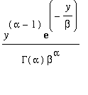
A continuous random variable is said to have a
gamma distribution with parameters
![]() ,
,
![]() if its
if its
pdf has the form: f(
y
) =
 if
y
> 0
0 if y <= 0
Here are some Gamma pdf graphs. Note that the maximum
shifts to the right and the peak value decreases as
![]() increases.
increases.
In the special case
![]() , the pdf is actually always decreasing for
y
> 0.
, the pdf is actually always decreasing for
y
> 0.
| > | f:=(y,alpha,beta)->y^(alpha-1)*exp(-y/beta)/(GAMMA(alpha)*beta^alpha); |

![]() = 1 :
= 1 :
| > | plot(f(y,1,1),y=0..10); |
![[Maple Plot]](images/Gamma8.gif)
![]() ,
,
![]() :
:
| > | plot(f(y,2,1),y=0..10); |
![[Maple Plot]](images/Gamma11.gif)
![]() ,
,
![]() :
:
| > | plot(f(y,3),y=0..10); |
![[Maple Plot]](images/Gamma14.gif)
![]() ,
,
![]() :
:
| > | plot(f(y,5),y=0..20); |
![[Maple Plot]](images/Gamma17.gif)
| > |