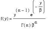
 for
y >=
0 (and 0 for
y
< 0)
MATH 375 -- Probability and Statistics 1
Gamma Distributions
October 29, 2003
Recall that we say Y has a Gamma distribution
if its pdf has the form
 for
y >=
0 (and 0 for
y
< 0)
| > | read "/home/fac/little/public_html/ProbStat/MaplePackage/MSP.map"; |
![]()
In our Maple package, the Gamma probability density function
is called GammaPDF -- it takes three parameters,
![]()
| > | GammaPDF(2,3,1.3); |
![]()
The Gamma distributions include distributions of various shapes,
skewed to different degrees always to the right.
The Gamma distribution with
![]() is a special case called
is a special case called
the exponential distribution. We looked at these already in an
example from class on Wednesday, 10/22. The exponential
pdf is always decreasing (a decaying exponential)
| > | plot(y->GammaPDF(1,2,y),0..10); |
![[Maple Plot]](images/Gamma6.gif)
When
![]() , the pdf has a local maximum at a positive
y.
, the pdf has a local maximum at a positive
y.
For instance, with
![]() , we have distributions like the following.
, we have distributions like the following.
Increasing the parameter
![]() stretches horizontally (hence shrinks
stretches horizontally (hence shrinks
vertically too to keep the total area = 1).
| > | plot(y->GammaPDF(2,1,y),0..20); |
![[Maple Plot]](images/Gamma10.gif)
| > | plot(y->GammaPDF(2,3,y),0..20); |
![[Maple Plot]](images/Gamma11.gif)
With
![]() ,
,
![]() , note that the peak has shifted to the right compared to
, note that the peak has shifted to the right compared to
![]()
and the overall distribution is more symmetrical.
| > | plot(y->GammaPDF(4,1,y),0..30); |
![[Maple Plot]](images/Gamma15.gif)
| > | plot(y->GammaPDF(4,3,y),0..30); |
![[Maple Plot]](images/Gamma16.gif)
Finally, with
![]() , we get something quite symmetrical.
, we get something quite symmetrical.
| > | plot(y->GammaPDF(50,1,y),0..120); |
![[Maple Plot]](images/Gamma18.gif)
The mean here is
![]() , and the variance is
, and the variance is
![]() . For comparison,
. For comparison,
here is the corresponding normal pdf plotted together with the Gamma pdf.
The Gamma pdf is skewed to the right compared to the normal.
| > | plot([y->NormalPDF(50,sqrt(50),y),y->GammaPDF(50,1,y)],20..120,color=[red,black]); |
![[Maple Plot]](images/Gamma21.gif)
| > |