MATH 375 -- Probability and Statistics 1

December 5, 2003

The joint density function for a bivariate normal

distribution.  Note this depends on 5 parameters

.   As we saw in class, the marginal

densities of   and   are normal and     are

the respective mean and standard deviation of the

two normal random variables (individually).

The parameter   actually equals the correlation

coefficient    .   The intuitive meaning

of   in this case is indicated by the following plots.

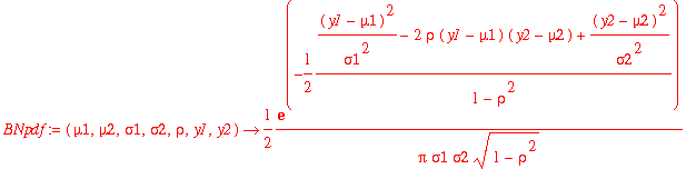
First we define the bivariate normal density function:

>	BNpdf:=(mu1,mu2,sigma1,sigma2,rho,y1,y2)->1/(2*Pi*sigma1*sigma2*sqrt(1-rho^2))*exp(-1/(1-rho^2)*((y1-mu1)^2/sigma1^2-2*rho*(y1-mu1)*(y2-mu2)+(y2-mu2)^2/sigma2^2)/2);

With   ,     are independent and the level curves the density function

are circles.

>	with(plots):

Warning, the name changecoords has been redefined

>	contourplot(BNpdf(0,0,1,1,0,y1,y2),y1=-3..3,y2=-3..3,scaling=constrained);

As   increases toward 1, the level curves become narrower and narrower

ellipses with major axis along a line through the point (  ) = (0,0)

here, with slope determined by the values of   

>	contourplot(BNpdf(0,0,1,1,.99,y1,y2),y1=-3..3,y2=-3..3,grid=[100,100],scaling=constrained);

>

>