MATH 304 -- Ordinary Differential Equations

November 2, 2000

Critical points and trajectories for the autonomous system:

There are four critical points of this system: (0,0), (0,3/2), (1,0), and (-1,2).

Here is a portion of the direction field and several approximate trajectories for

the system:

> with(DEtools):

> phaseportrait({diff(x(t),t)=x(t)-x(t)^2-x(t)*y(t),diff(y(t),t)=3*y(t)-x(t)*y(t)-2*y(t)^2},[x(t),y(t)],t=0..3,[[x(0)=-.3,y(0)=.1],[x(0)=.3,y(0)=.2],[x(0)=-0.5,y(0)=2],[x(0)=-1,y(0)=2.2],[x(0)=1,y(0)=1],[x(0)=-.1,y(0)=.1],[x(0)=.5,y(0)=0],[x(0)=3,y(0)=.01],[x(0)=3,y(0)=-0.01],[x(0)=-.1,y(0)=-.1],[x(0)=.1,y(0)=-.1]],x=-2..2,y=-2..3,linecolor=blue,stepsize=0.01);

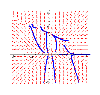
From this, it appears reasonable that:

(0,0) is a node (a "source")

(1,0) and (-1,2) are saddle points

(0,3/2) is another node (a "sink")

Today we want to start to address the question: Given just the ODE's in the system,

is it possible to determine the types of the critical points without plotting

the direction field and approximate trajectories?

The linearization of our system at (0,0) is obtained by ignoring all

quadratic (and higher order) terms in the Taylor expansions of

at the critical point. Here we get

when we linearize at (0,0).

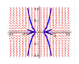
Comparing the linearization at (0,0) to a "zoomed" portion of the phase portrait

near (0,0) (we plot only x, y in [-0.2,0.2] x [-0.2, 0.2]. The linearization first:

> phaseportrait({diff(x(t),t)=x(t),diff(y(t),t)=3*y(t)},[x(t),y(t)],t=0..1,[[x(0)=.03,y(0)=.01],[x(0)=-.03,y(0)=.01],[x(0)=.03,y(0)=.001],[x(0)=-.03,y(0)=.001],[x(0)=.03,y(0)=-.01],[x(0)=-.03,y(0)=-.01],[x(0)=.03,y(0)=-.001],[x(0)=-.03,y(0)=-.001]],x=-0.2..0.2,y=-0.2..0.2,linecolor=blue,stepsize=0.001);

Now the trajectories of the full non-linear system starting from the same initial points:

> phaseportrait({diff(x(t),t)=x(t)-x(t)^2-x(t)*y(t),diff(y(t),t)=3*y(t)-x(t)*y(t)-2*y(t)^2},[x(t),y(t)],t=0..1,[[x(0)=.03,y(0)=.01],[x(0)=-.03,y(0)=.01],[x(0)=.03,y(0)=.001],[x(0)=-.03,y(0)=.001],[x(0)=.03,y(0)=-.01],[x(0)=-.03,y(0)=-.01],[x(0)=.03,y(0)=-.001],[x(0)=-.03,y(0)=-.001]],x=-0.2..0.2,y=-0.2..0.2,linecolor=blue,stepsize=0.001);

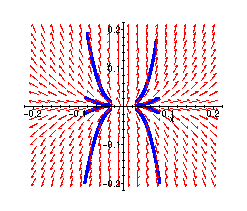
These two plots are almost indistinguishable!!

Similarly, zooming in near the critical point at (-1,2) (translated to the origin)

> phaseportrait({diff(u(t),t)=u(t)+v(t),diff(v(t),t)=-2*u(t)-4*v(t)},[u(t),v(t)],t=0..2,[[u(0)=.01,v(0)=.2],[u(0)=-.1,v(0)=.2],[u(0)=.1,v(0)=-.2],[u(0)=-.01,v(0)=-.2]],u=-0.2..0.2,v=-0.2..0.2,linecolor=blue,stepsize=0.001);

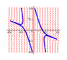
> phaseportrait({diff(u(t),t)=u(t)+v(t)-u(t)^2-u(t)*v(t),diff(v(t),t)=-2*u(t)-4*v(t)-u(t)*v(t)-2*v(t)^2},[u(t),v(t)],t=0..2,[[u(0)=.01,v(0)=.2],[u(0)=-.1,v(0)=.2],[u(0)=.1,v(0)=-.2],[u(0)=-.01,v(0)=-.2]],u=-0.2..0.2,v=-0.2..0.2,linecolor=blue,stepsize=0.001);

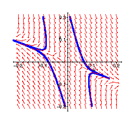
The two plots again agree quite closely.