MATH 304 -- Ordinary Differential Equations

Solutions -- Lab 3

November 6, 2000

A)

> aux:=2*10^(-6)*r^2+10^(-3)*r+1;

> fsolve(aux,r,complex);

> v1:=t->exp(-250*t)*cos(661.4378278*t);

> v2:=t->exp(-250*t)*sin(661.4378278*t);

> vp:=t->A*cos(50*t)+B*sin(50*t);

> 2.0*10^(-6)*diff(vp(t),t$2)+1.0*10^(-3)*diff(vp(t),t)+vp(t);

> ABsol:=fsolve({.995*A+.05*B,-.05*A+.995*B-20},{A,B});

> vpp:=t->subs(ABsol,vp(t));

> vC:=t->c1*v1(t)+c2*v2(t)+vpp(t);

> vC(t);

> initeqs:={vC(0)=0,subs(t=0,diff(vC(t),t))=1};

> cvals:=fsolve(initeqs,{c1,c2});

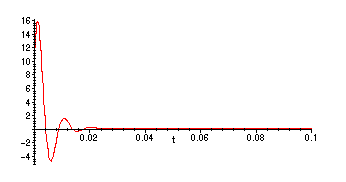
The transient terms die away to zero very quickly in this example:

> plot(10*v1(t)+20*v2(t),t=0..0.1);

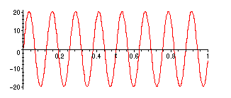
> plot(subs(cvals,vC(t)),t=0..1);

B)

The case R = 0

If is not a root of the auxiliary equation, the general solution is:

> vnonres:=t -> c1*cos(t/sqrt(L*C))+c2*sin(t/sqrt(L*C))+a/(1-omega^2*L*C)*sin(omega*t);

If is a root of the auxiliary equation, then the general solution is

> vres:=t->c1*cos(t/sqrt(L*C))+c2*sin(t/sqrt(L*C))-a/(2*sqrt(L*C))*t*cos(omega*t);

C)

For the first two cases here, and ,

is not a root of the auxiliary equation, so we use the first form from question B:

> C:=1.0*10^(-6); L:=1; a:=1;

> vres(t);

> vnonres(t);

> omega:=900;

> initeqs1:={vnonres(0)=1,subs(t=0,diff(vnonres(t),t))=0};

> sol1:=fsolve(initeqs1,{c1,c2});

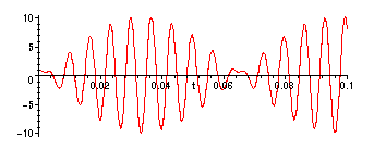
> plot(subs(sol1,vnonres(t)),t=0..0.1);

>

> omega:=950;

> initeqs2:={vnonres(0)=1,subs(t=0,diff(vnonres(t),t))=0};

> sol2:=fsolve(initeqs2,{c1,c2});

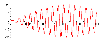
> plot(subs(sol2,vnonres(t)),t=0..0.1);

does give a root of the auxiliary equation so we need to

use the second form of solution from question B

> omega:=1000;

> initeqs3:={vres(0)=1,subs(t=0,diff(vres(t),t))=0};

> sol3:=fsolve(initeqs3,{c1,c2});

> plot(subs(sol3,vres(t)),t=0..0.2);

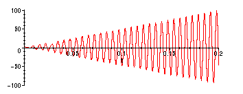
This is the resonant solution -- the amplitude of the oscillations is increasing without

bound as t increases.

The final two cases are like the first two:

> omega:=1050;

> initeqs4:={vnonres(0)=1,subs(t=0,diff(vnonres(t),t))=0};

> sol4:=fsolve(initeqs4,{c1,c2});

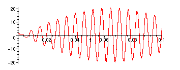
> plot(subs(sol4,vnonres(t)),t=0..0.1);

>

> omega:=1100;

> initeqs5:={vnonres(0)=1,subs(t=0,diff(vnonres(t),t))=0};

> sol5:=fsolve(initeqs5,{c1,c2});

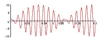
> plot(subs(sol5,vnonres(t)),t=0..0.1);

D) If R > 0, then roots of the auxiliary equation are

r =

r =

The real part is always negative in both, so all solutions tend to zero as .

Get real solutions only if

E)

> R:=2000.; C:=2.0*10^(-7); L := 1.5; omega:='omega';

> aux:=L*C*r^2+R*C*r+1;

> fsolve(aux,r,complex);

> v1:=t->exp(-666.6666667*t)*cos(1699.673171*t);

> v2:=t->exp(-666.6666667*t)*sin(1699.673171*t);

Again, the transients (the homogeneous solution terms) will die away so quickly that the

particular solution determines the shape for large t. The particular solution in this

case always has the form since neither of these

terms solves the homogeneous equation if R is not zero (all solutions of the homogeneous

equation contain a decaying exponential by question D).

> vp:=t->A*sin(omega*t)+B*cos(omega*t);

> ss:=L*C*diff(vp(t),t$2)+R*C*diff(vp(t),t)+vp(t);

> a:='a';

> collect(ss,{cos(omega*t),sin(omega*t)});

> ABsol:=solve({-.3000000000e-6*B*omega^2+.4000000000e-3*A*omega+B,-.3000000000e-6*A*omega^2-.4000000000e-3*B*omega+A=a},{A,B});

> vpp:=t->subs(ABsol,vp(t));

The long-term behavior is determined by the particular solution, so as a

"short-cut" we only plot that (!!!!!!)

For different from the frequency of the homogenous solution, the particular

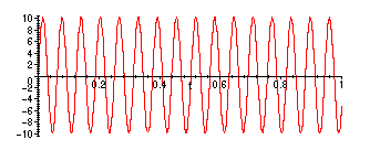
solutions will look like a sinusoid with amplitude roughly a, frequency

> omega:=100; a:=10;

> plot(vpp(t),t=0..1);

If or so (the frequency of the homogenous solutions), then something interesting happens:

> omega:=1699.67; a;

> plot(vpp(t),t=0..0.1);

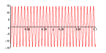
Note that the amplitude here is significantly larger than the amplitude of the forcing term: .

If , larger than the frequency of the homogeneous solutions, then something else happens:

> omega:=3000: plot(vpp(t),t=0..0.01);

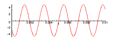
Here the amplitude is much smaller than 10; the frequency is also much larger, so we have

plotted a smaller piece of the solution.

In fact, we can plot the amplitude of the particular solution as a function of the forcing frequency

, as follows. The particular solution is

> vpp(t);

which has the form AA cos( ) + BB sin( ). Every such function is a sinusoid,

with amplitude

> AA:=coeff(vpp(t),sin(omega*t)):

> BB:=coeff(vpp(t),cos(omega*t)):

To plot, we take a = 1:

> a:=1;

> amp:=simplify(sqrt(AA^2+BB^2));

> plot(amp(omega),omega=0..5000);

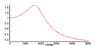
There is resonance in the sense that the amplitude of the longterm solution can be larger

than the amplitude of the forcing term, but the solution is always bounded, unlike the R = 0 case.