Lab2Results.html

Analysis and Comparison of the Five Proposals for Heating

Plans for Smith Hall, Holy Cross College

Notes:

1) In preparing this comparison, we looked at solutions of the model ODE's

starting from T(0) = 70 in all cases.

2) Also, the heat source term for the building was given in degrees per hour,

not degrees per day. Hence the heat source term was changed from .1 to 2.4 in

many cases.

This means that the estimates and solutions below will vary slightly from those proposed.

&&&&&&&&&&&&&&&&&&&&&&&&&&&&&&&&&&&&&&&&&&&&&

RESULTS OF COMPETITION:

Proposals I and V are similar in that they attempt to trade cold temperatures in the

building through the winter months for lower costs. Unfortunately, having an

office/classroom building at below 60 or between 62 and 64 degrees for extended

periods is not acceptable to most people, so we must reject those plans.

Of the remaining proposals, even though it attains the tightest temperature control,

Proposal II is by far the most expensive, so we must also reject it.

Proposal III achieves good temperature control with reasonable cost using

proportional controls, but is outperformed by the remaining method.

Proposal IV uses a very effective modification of the basic "bang-bang" control

strategy (only applying heating/air conditioning when the temperature gets

outside the band 68 to 72 degrees F). This method achieves by far the best combination

of temperature control and low cost.

The Winner is: Plan IV (Curtis, Dolley, Germino, Grande) for excellent cost and

temperature control, also best estimate of total cost (although the estimated

cost is probably very high -- I do not understand why it came out that way; see

the results below.)

Congratulations!!

&&&&&&&&&&&&&&&&&&&&&&&&&&&&&&&&&&&&&&&&&&&&&&&

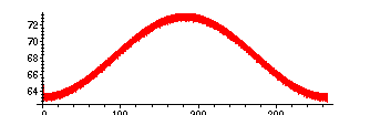
Proposal I: Beattie, Broadbent, Camarra, Carbonneau

Use Proportional controls with

> restart;

> read `/home/fac/little/public_html/ODE00/RK4.map`:

> FI := (t,T)-> evalf(-.424*(T(t)-(8*sin(2*Pi*t)-27.5*cos(2*Pi*t/365)+52.5))+ 2.4 + 2*(70-T(t))):

> solI:=RungeKutta(FI,0,70,365,3650):

> plot(solI);

Then the total heating cost will be:

Explanation: The integral of the control term: from 0 to 365 gives the total

heating/cooling your plan applies. The units are degrees. Multiplying by 30

(cost in dollars for each degree) gives the total cost for the whole year. We estimated the cost

with a left-hand Riemann sum with = 1/10 day:

> 30*2*add(abs(solI[j][2]-70)*(1/10),j=1..3650);

That is, about $73 thousand for the year estimated cost.

&&&&&&&&&&&&&&&&&&&&&&&&&&&&&&&&&&&&&&&&&&&&&&&&&&&

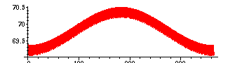
Proposal II: Kavanagh, Macholz, Mannix

Use Proportional controls with

> restart;

> read `/home/fac/little/public_html/ODE00/RK4.map`;

> FII := (t,T)-> evalf(-.424*(T(t)-(8*sin(2*Pi*t)-27.5*cos(2*Pi*t/365)+52.5))+ 2.4 + 20*(70-T(t)));

> solII:=RungeKutta(FII,0,70,365,3650):

> plot(solII);

Then the total heating cost will be:

Explanation: The integral of the control term: from 0 to 365 gives the total

heating/cooling your plan applies. The units are degrees. Multiplying by 30

(cost in dollars for each degree) gives the total cost for the whole year. We estimated the cost

with a left-hand Riemann sum with = 1/10 day:

> 30*20*add(abs(solII[j][2]-70)*(1/10),j=1..3650);

That is, about $89 thousand for the year estimated cost.

&&&&&&&&&&&&&&&&&&&&&&&&&&&&&&&&&&&&&&&&&&&&&&&&&&&

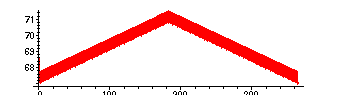
Proposal III: Sexton, Sparks, Sullivan

Use Proportional controls with U(t,T) = 5.75 (70 - T)

> restart;

> FIII:=(t,T)-> evalf(-(.424)*(T(t) - (80-(110/365)*abs(182.5-t)+8*sin(2*Pi*t)))+ 2.4 + 5.75*(70-T(t)));

> read `/home/fac/little/public_html/ODE00/RK4.map`;

> solIII:=RungeKutta(FIII,0,70,365,3650):

> plot(solIII);

Then the total heating cost will be:

Explanation: The integral of the control term: from 0 to 365 gives the total

heating/cooling your plan applies. The units are degrees. Multiplying by 30

(cost in dollars for each degree) gives the total cost for the whole year. We estimated

the integral with a left-hand Riemann sum with = 1/10 day

> 30*5.75*add(abs(solIII[j][2]-70)*(1/10),j=1..3650);

That is, about $72 thousand for the year estimated cost.

&&&&&&&&&&&&&&&&&&&&&&&&&&&&&&&&&&&&&&&&&&&&&&&

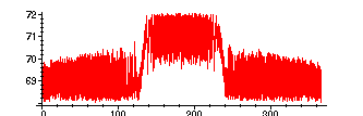
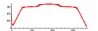
Proposal IV: Curtis, Dolley, Germino, Grande

Use (modified) "bang-bang" controls with

U(t,T) = 50 if T < 68, -50 if T > 72, and no heating/AC if 68 <= T <= 72

Model:

> restart;

> A := t -> piecewise(t<182, (80-55*(182-t)/182) - 8*cos(2*Pi*t),t>182,(80-55*(t-182)/182) - 8*cos(2*Pi*t));

> FIV := proc(t,T) if T < 68 then RETURN(evalf(-.423*(T-A(t))+2.4+50)) elif T > 72 then RETURN(evalf(-.423*(T-A(t))+2.4-50)) else RETURN(evalf(-.423*(T-A(t))+2.4)) fi end:

> read `/home/fac/little/public_html/ODE00/RK4.map`;

> solIV:=RungeKutta(FIV,0,70,365,3650):

> plot(solIV);

To estimate the total cost of this plan, we used the approximate values for the solution

function produced by the RungeKutta procedure.

The total heating cost will be:

(Explanation: The integral of the control term: from 0 to 365 gives the total

heating/cooling your plan applies. The units are degrees. Multiplying by 30

(cost in dollars for each degree) gives the total cost for the whole year.)

We estimated the integral with a left-hand Riemann sum with = 1/24 day, computed by

a modified version of the Runge-Kutta procedure:

> UIV := proc(T) if T < 68 then RETURN(50) elif T > 72 then RETURN(-50) else RETURN(0) fi end:

> read `/home/fac/little/Classes/ODE00/RKBBCost.map`;

> RKBBCost(FIV,UIV,0,25,365,365*24);

That is, about $2 thousand for the year estimated cost, by this method of computing

the cost.

A similar computation, but using the Euler method to approximate values of the

solution T(t). This is equivalent to what your FORTRAN program does,

but written in Maple. I cannot explain the discrepancy between this result and

yours(!!!!!)

> read `/home/fac/little/Classes/ODE00/EulerBBCost.map`;

> EulerBBCost(FIV,UIV,0,25,365,365*24);

That is, about $71 thousand for the year estimated cost.

Note: I do not know why your cost estimate, also generated by an Euler-like method,

is roughly twice as large. I have spent a lot of time looking at it without success(!) Numerical

approximations can be quite tricky.

The thing I can say is that the Runge-Kutta method should be giving more accurate estimates

of the actual temperature, so that the actual cost is probably between these estimates, and

quite small compared to the other plans. We have a winner!!!!!!!!!!!!!!!!!!!

&&&&&&&&&&&&&&&&&&&&&&&&&&&&&&&&&&&&&&&&&&&&&&&&&&&&

Proposal V: Basile, Marani, Paukert, Richard

Use "bang-bang" controls with

U(t,T) = 10 if T < 70, -10 if T > 70, and no heating/AC if T = 70

Model:

> restart;

> A := t -> piecewise(t<=182,.302*t+25+8*sin(2*Pi*t),t>182,-.299*t+134.4 + 8*sin(2*Pi*t));

> FV := proc(t,T) if T < 70 then RETURN(evalf(-.424*(T-A(t))+2.4+10)) elif T > 72 then RETURN(evalf(-.424*(T-A(t))+2.4-10)) else RETURN(evalf(-.423*(T-A(t))+2.4)) fi end:

> read `/home/fac/little/public_html/ODE00/RK4.map`;

> solV:=RungeKutta(FV,0,70,365,3650):

> plot(solV);