MATH 304 -- Ordinary Differential Equations
Some examples for the heating/cooling discussion lab.
To deal with control terms in ODE's that depend on the
value of the dependent variable, but not continuously, it is
sometimes necessary to use a procedure to compute values
of the slope function. For instance, suppose we wanted to
generate approximate solutions of
dy/dx = F(x,y),
where F(x,y) = x + y if y < 10
x - 2y if y >= 10
Since F(x,y) is discontinuous along the line y = 10, our
Existence and Uniqueness Theorem does not apply once
a solution crosses that line. ("All bets are off" about whether
a solution even exists then!) We can still try to apply an
approximate numerical method, though, to try to get a feeling
for what is going on. To do that, we could start by defining a
Maple function that computes F as follows:
> F := proc(x,y) if y < 10 then RETURN(x+y) else RETURN(x-2*y) fi end:
Unfortunately, the built-in DEplot command in Maple apparently
cannot handle a slope function like this one (or at least I have not
been able to make it do so!) Fortunately, there is another way to
proceed. We begin by reading in Maple code for an approximate
numerical method called the Runge-Kutta method (similar to the
method Maple uses to plot approximate solutions of ODE).
> read `/home/fac/little/public_html/ODE00/RK4.map`;
The command defined in this file has the format
RungeKutta(F,t0,y0,tf,numpoints);
where:
F is the slope function for the ODE you want to solve (this should
be the name of a procedure or function that computes the slope value).
It should be a function of two variables, with the independent variable
first in the list of variables.
t0 is the initial value of the independent variable (t)
y0 is the initial value of the dependent variable (y)
tf is the final value of the independent variable (you'll get approximate
solution values for t0 <= t <= tf
numpoints is the number of values of the independent variable that will
be computed (stepsize = (tf - t0)/numpoints)
The output from this is a list of points (approximations to points on the
graph of the solution with the initial conditions. You can plot the points
just by giving the list as input to the plot command. (Maple generates
the plot by connecting the points by straight line segments -- exactly what
DEplot does too, by the way!)
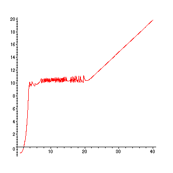
Here's an example: We plot the solution of the above ODE with initial
condition y(1) = -1 for 1 <= x <= 40, using numpoints = 500
> sol:=RungeKutta(F,1,-1,40,500):
> plot(sol);

>
To make sure you understand this plot, ask yourself: Why does it have this shape???