MATH 371 -- Numerical Analysis
October 15 -- Polynomial Interpolation, Cubic Spline Interpolation
For "nice" functions like cos( x ) on small intervals, we can see that
the error of interpolation -> 0 as n ->
![]() . For instance, using the
. For instance, using the
bound
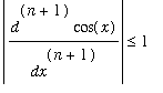 , the following is an upper bound on the
interpolation error using the n th degree polynomial:
> CosErrorBound:=(n,x)->1/(n+1)!*product(abs(x-j/n),j=0..n);
The larger n is, the smaller this error bound is:
> plot(CosErrorBound(5,x),x=0..1);
![[Maple Plot]](images/ErrInterp24.gif)
> plot(CosErrorBound(10,x),x=0..1);
![[Maple Plot]](images/ErrInterp25.gif)
> plot(CosErrorBound(20,x),x=0..1);
![[Maple Plot]](images/ErrInterp26.gif)
Note the scales on the y- axes(!) If we plot the interpolating polynomial together with
cos( x ) on [0,1], the difference is already invisible with n = 5:
> with(CurveFitting):
> IP:=x->PolynomialInterpolation([seq(evalf(j/5),j=0..5)],[seq(evalf(cos(j/5)),j=0..5)],x);
![]()
![]()
> plot({IP(x),cos(x)},x=0..1);
![[Maple Plot]](images/ErrInterp29.gif)
If the interval is not small, and/or the function is not "nice", then the
picture can be entirely different.
Next, let's try an interpolating polynomial for
![]() , which is "nice" by almost
, which is "nice" by almost
any criterion. BUT, let's use x = 1,2,3,4,5, so the interval is not so small.
There are n + 1 = 5 points, so n = 4:
> IP2:=x->PolynomialInterpolation([1.,2.,3.,4.,5.],[exp(1.),exp(2.),exp(3.),exp(4.),exp(5.)],x);
![]()
To see how closely our interpolating polynomial matches the exponential function at other points we can either compute a few values:
> IP2(1.35); exp(1.35);
![]()
![]()
> IP2(1.62); exp(1.62);
![]()
![]()
Note the agreement is not so close any more!
The actual error versus the theoretical error bound for polynomial interpolation in this case,
using the upper bound M =
![]() for the 5th derivative of
for the 5th derivative of
![]() on [1,5]:
on [1,5]:
> plot({abs(exp(x)-IP2(x)),abs((exp(5)/120)*(x-1)*(x-2)*(x-3)*(x-4)*(x-5))},x=1..5,y=0..5);
![[Maple Plot]](images/ErrInterp218.gif)
In this case again, taking more interpolation points will help, though
> ExpErrorBound:=(n,x)->abs(exp(5)/(n+1)!*product(x-(1+4*(j/n)),j=0..n));
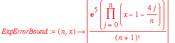
> plot(ExpErrorBound(10,x),x=1..5);
![[Maple Plot]](images/ErrInterp220.gif)
And taking
n ->
![]() will make the error bound go to zero on the whole
will make the error bound go to zero on the whole
interval.
Other shapes of graphs are just very difficult for polynomials to approximate
well . An example is graphs with horizontal asymptotes, if we take a large
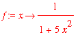
interval. For instance, if we wanted to interpolate a function like:
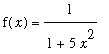
> f:=x->1/(1+5*x^2);
> xlist:=n->[seq(evalf(-3+6*j/n),j=0..n)];
![]()
> ylist:=n->map(f,xlist(n));
![]()
> xlist(10);
![]()
![]()
> ylist(10);
![]()
![]()
> IP3:=n->PolynomialInterpolation(xlist(n),ylist(n),x);
![]()
Here are the interpolating polynomials of degrees 4,8,12,16 plotted together with y = f( x ):
> plot({f(x),IP3(4)},x=-3..3);
![[Maple Plot]](images/ErrInterp231.gif)
> plot({f(x),IP3(8)},x=-3..3);
![[Maple Plot]](images/ErrInterp232.gif)
> plot({f(x),IP3(12)},x=-3..3);
![[Maple Plot]](images/ErrInterp233.gif)
> plot({f(x),IP3(16)},x=-3..3);
![[Maple Plot]](images/ErrInterp234.gif)
>
In fact, we can see that the error near the ends of the interval is growing with n,
not decreasing. The technical name for this phenomenon is `` polynomial wiggle ''.
One "way around" these problems is to use a different approach to interpolation.
Instead of trying to use a single polynomial of high degree to approximate a function
like this over a large interval, it certainly seems to be better to use a piecewise-polynomial
function -- one defined by different polynomial formulas on different segments of its
domain. One of the most popular choices here is to use ``cubic splines'' -- piecewise
cubic polynomial functions. We will see in class next time that there is enough freedom
in cubic polynomials to be able to construct a function
![]() defined by cubics
defined by cubics
![]() on [
on [
![]() ] for i = 0,1,2, ... , n-1, satisfying:
] for i = 0,1,2, ... , n-1, satisfying:
1)
![]() ,
,
![]() = f(
= f(
![]() ) for
i
= 1, ...,
n
-1, and
) for
i
= 1, ...,
n
-1, and
![]()
so
![]() is a continuous function interpolating the points (
is a continuous function interpolating the points (
![]() ),
i
= 0, 1, ... ,
n,
),
i
= 0, 1, ... ,
n,
2)
S'
(
x
) is continuous -- the derivative of
![]() at
at
![]() is the same as the derivative
is the same as the derivative
of
![]() at
at
![]() for
i =
0,1,...,
n
-2
for
i =
0,1,...,
n
-2
3)
S''
(
x
) is continuous -- the second derivative of
![]() at
at
![]() is the same as the
is the same as the
second derivative of
![]() at
at
![]() for
i =
0,1,...,
n
-2, and
for
i =
0,1,...,
n
-2, and
4)
Either:
S''
(
![]() ) = 0 and
S''
(
) = 0 and
S''
(
![]() ) = 0 (``free or natural spline''),
or
) = 0 (``free or natural spline''),
or
S'
(
![]() ) =
a
and
S'
(
) =
a
and
S'
(
![]() ) =
b
for arbitrary
a, b
(``clamped spline'')
) =
b
for arbitrary
a, b
(``clamped spline'')
The CurveFitting package also contains a routine that computes free cubic splines. Here
is a first example, using the same function and the same interpolation points as in the
last examples. The output shows the piecewise cubics:
> IS:=x->Spline(xlist(10),ylist(10),x);
![]()
> plot({IS(x),f(x)},x=-3..3);
![[Maple Plot]](images/ErrInterp257.gif)
>
Note that the results do not show the same kind of ``wiggle problems'' that the
high degree interpolating polynomials showed(!)