MATH 241, section 1 -- Multivariable Calculus 

The "Method of Slices"
September 3, 2010

Let's consider using slices to study the shape of the surface in  `*`(`^`(real, 3))  defined
by the equation   `+`(`*`(`^`(x, 2)), `*`(`^`(y, 2)), `-`(`*`(`^`(z, 2))), `-`(1)) = 0.  

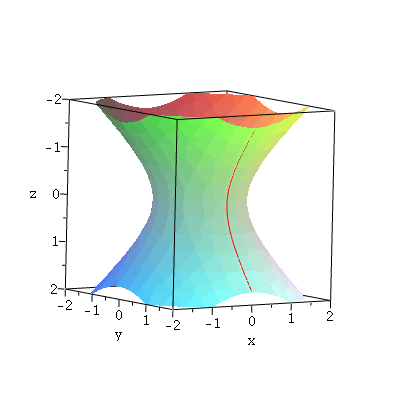
First, the slice in the plane  x = 0-- the slice is the curve on the surface
shown in red:with(plots); -1


`assign`(SP, implicitplot3d(`+`(`*`(`^`(x, 2)), `*`(`^`(y, 2)), `-`(`*`(`^`(z, 2))), `-`(1)), x = -2 .. 2, y = -2 .. 2, z = -2 .. 2, grid = [20, 20, 20], axes = boxed, style = surface)); -1
 

`assign`(CP1, spacecurve({[0, `+`(`-`(cosh(t))), sinh(t), t = -1.3 .. 1.3], [0, cosh(t), sinh(t), t = -1.3 .. 1.3]}, color = red)); -1
 

display(SP, CP1); 1 

Plot_2d
 

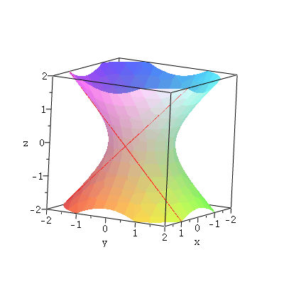
Now the slice in the plane  x = 1; -1 

`assign`(CP2, spacecurve({[1, t, t, t = -2 .. 2], [1, t, `+`(`-`(t)), t = -2 .. 2]}, color = red)); -1 


display(SP, CP2); 1 

Plot_2d
 

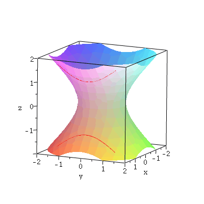
Finally, the slice in the plane  x = 1.5; -1 


`assign`(CP3, spacecurve({[1.5, `*`(sqrt(`+`(`^`(1.5, 2), `-`(1))), `*`(sinh(t))), `*`(sqrt(`+`(`^`(1.5, 2), `-`(1))), `*`(cosh(t))), t = -1 .. 1], [1.5, `*`(sqrt(`+`(`^`(1.5, 2), `-`(1))), `*`(sinh(t...
 

display(SP, CP3); 1 

Plot_2d
 

The first and the third curve are both hyperbolas in those planes but note how 

the shape changes as we go through the slice in the plane  x = 1.