MATH 241 -- Multivariable Calculus
Constrained Optimization and Lagrange Multipliers
November 2, 2010
Consider the problem of optimizing ![]() at the
at the
points of the ``constraint curve''
![]()
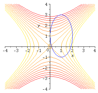
Here is a picture of the constraint curve superimposed on the
contour plot of the function f
| > |
| > |
| > |
| > |
 |
Think of the contour plot here as the map of a landscape. The constraint
curve might then describe a hike we are taking through the landscape.
The question we want to answer is:
At which point(s) did we reach a maximum elevation on the hike,
and where did we reach a minimum elevation?
In this case we can parametrize the constraint curve easily since it is an ellipse
with center at (1,1) semimajor axis 2 parallel to the y-axis, and semiminor
axis 1 parallel to the x-axis:
![]()
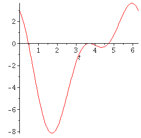
If we substitute the coordinate functions from this into f (x, y), then we can
see explicitly where ![]() achieves its greatest and smallest values:
achieves its greatest and smallest values:
| > |
 |
Note how this plot relates to what we see in the first plot of the constraint curve
and the contours. There is an interesting geometric relation between the constraint
curve and the contour whenever we ``hit'' a critical point of the function ![]() restricted to the contour. Can you see what it is?
restricted to the contour. Can you see what it is?
The example, continued
One way to say the relation is that the contour of ![]() and the constraint
and the constraint
curve are tangent to each other at each of those points. (That is, the two
curves have the same tangent line!)
This observation holds in general for the following reason. Suppose that we
can parametrize a portion of the constraint curve near a point ![]() where
where
the restriction of ![]() has a critical point as a curve
has a critical point as a curve ![]() . (This is always
. (This is always
possible when ![]() by a more advanced result called the Implicit
by a more advanced result called the Implicit
Function Theorem.) Say ![]() If the restricted function has a
If the restricted function has a
critical point at ![]() , then
, then
![]() at
at ![]() However, by the multivariable Chain Rule we discussed earlier, this implies
However, by the multivariable Chain Rule we discussed earlier, this implies
![]() In other words, the gradient vector of f at
In other words, the gradient vector of f at ![]() is orthogonal to the tangent
is orthogonal to the tangent
line to the constraint curve at that point. Since the gradient vector of g at
that point is also orthogonal to the tangent line to the constraint curve,
we have that the two vectors ![]() and
and ![]()
![]()
(called a Lagrange multiplier ) such that
![]()
Hence we get the ``method of Lagrange multipliers" for solving the constrained
optimization problem:
1. Set up the Lagrange equations :
![]()
![]()
2. Solve them simultaneously for x, y, (and sometimes λ)
3. By comparing the values of f at all of the points
found in step 2, we can determine the
maximum and minimum values of f on the constraint curve.
(Note: it is often the case that the values of λ in the
solutions of the Lagrange equations are not relevant,
and we will not use them for anything. Still, there are
times when it might be convenient to solve for λ
and use those values to get x and y.
Here is how this ``program'' works in our example above:
1. The Lagrange equations are
![]() The hardest step is almost always actually solving
The hardest step is almost always actually solving
the Lagrange equations. A good general strategy is
to try to use the equations to eliminate variables and
reduce down to an equation in one variable (if possible).
For some equations, though, this may require a good deal
of cleverness to carry through. This is an example where
that is the case.
Here note that the first two equations allow us to
eliminate λ:
![]()
![]()
So ![]()
![]() Then we can eliminate the x in the constraint
Then we can eliminate the x in the constraint
equation by substituting for the ![]()
![]()
So
![]()
| > |
| (1.1) |
| > |
| (1.2) |
So this is a ``hard'' example where there are no rational roots and
where using a numerical root-finding method is probably needed.
The Maple command for this is the fsolve command. To set up
for the fact that there are several different y - values. We collect
them in a list:
| > |
| (1.3) |
For each of these y - values, there is exactly one corresponding x - value,
given by ![]() We can have Maple do all the calculations for us like this, using
We can have Maple do all the calculations for us like this, using
the ``for loop'' structure to build up a corresponding list of x-values.
| > |
Next, we print out the 4 points and the values of f at each one:
| > |
| (1.4) |
So we see that
the maximum value of f on the constraint curve is about 3.66, achieved at the
third critical point in this list: [![]() ] , and
] , and
the minimum value is about - 8.14, achieved at the last one: ![]() .
.
Note how this agrees with our graph of the restriction of f to the constraint set
before(!) The two other points give a local minimum and a local maximum that are not
global extrema on the constraint curve.