MATH 241 -- Multivariable Calculus 

Differentiability for October 20, 2010 

We have now introduced directional derivatives of    in all 

directions  at points   and seen the special cases  

and   that give the partial derivatives:
We will next consider the following question:  Is there some  

single object that we can consider as ``the (total) derivative of  f " 

at We will see that the answer is yes, but the exact form 

and the way this appears as a derivative is going to take some explanation. 

This is perhaps the area where the ideas from  1-variable  calculus need 

to be augmented the most to deal with functions of several variables. 

To prepare for this, let's go back and reconsider what it means for a  

function of one variable,  to be differentiable  from a viewpoint 

that might be new to you.  The way you have probably seen this idea 

defined in your previous calculus courses is this:  is said to be  

differentiable at  if the limit 

exists and if it does, then this limit computes the value of  the derivative  

The equation  

can be rearranged to
 

If we rewrite  then  and   

Therefore this last equation can be rewritten as 

What does this really mean?  Well, note that the top is   

where  is the linear function whose 

graph is the  tangent line to  at  Not only is   

as  In fact, it is going to zero faster than  

in the sense that the quotient is still going to zero after we divide 

by  Intuitively, we can factor    out of the top and  

cancel with the bottom and what is left is still going to zero as  In graphical terms, this means that when  exists, the graph  

gets very close to the tangent line if we ``zoom in'' on the point  

in a suitable way.  Here is an example to show what this means. 

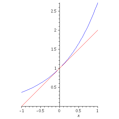
We know  is differentiable at   and  

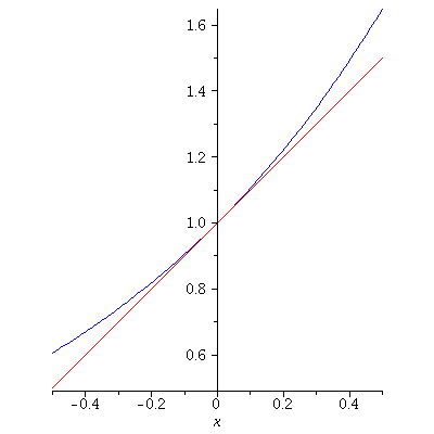
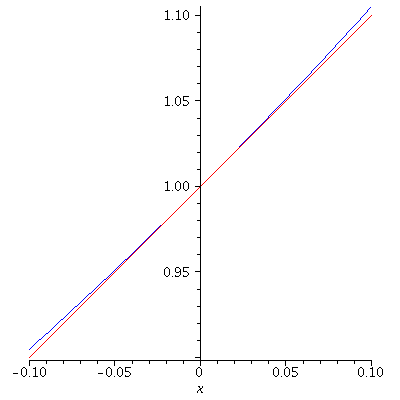
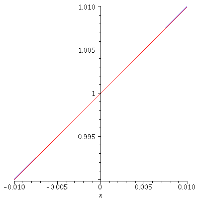
Hence  Here is the graph   

together with the tangent line plotted over smaller and smaller intervals. 

Note how the graph quickly becomes indistinguishable from the tangent 

line (up to the resolution of the screen): 

>

 

>

 

>

 

>

 

Here is the plot of  which indicates how the limit (*) above works in this case. 

>

 

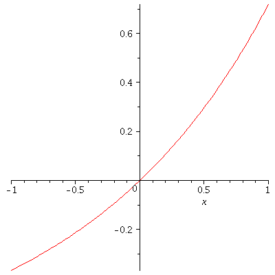This certainly seems to approach  0  as  (This can also be shown, of course, via techniques including 

L'Hopital's Rule for limits.) 

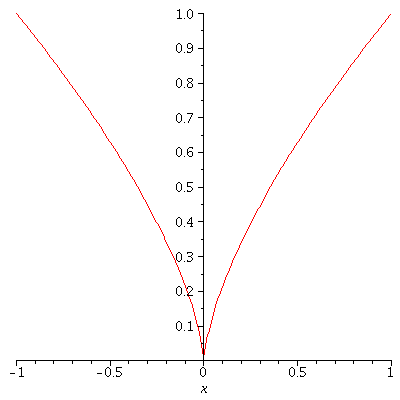
On the other hand, here is a function  and an  where  does not exist. 

>

 

Note what happens if we plot  for any real   

>

 

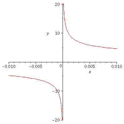We can see  

                                                 while    no matter what the value of   a  is. 

Intuitively, no straight line passing through  (0,0) approximates the shape of the graph  at all well near   (0,0).  

It is this idea of differentiability that extends well to functions of several variables: 

Intuitively, we say  is differentiable  at if there is some linear function  

graph z = approximates the graph  

z = well near More precisely,  we say  is differentiable  at if there is some linear function  

In fact there is only one "candidate" for the linear function:  It is possible to see that  

in   








is a plane in  So the question
we're asking is really -- does that plane approximate the shape of the graph
well near  
Example 1.   Let  We claim that    is differentiable at   

We have  and  First, we plot  and  together to see whether it looks like the plane is approximating the graph well.

We plot the graphs of  f, ℓ  together on a small rectangle with  (1,2)  at the 

center: 

>

 

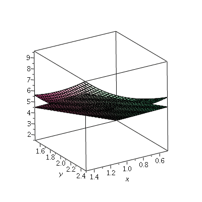This looks pretty good, and it would look progressively better as we zoomed in towards 

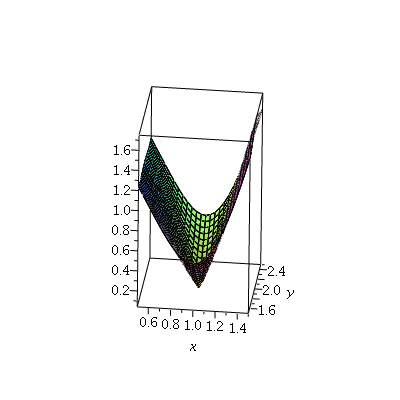
The next plot shows what happens if we graph the function



again on a small rectangle with (1,2) at the center:

 

>

 

In fact, it is a theorem that if  and its two first order partial derivatives  and  are continuous
on some open set U  in containing  then  is differentiable at  That theorem applies
in this example, since   are all polynomial functions. 

(Recall polynomials in  x, y are continuous at all points in  Next, we want to see what can "go wrong" if   f  is not differentiable at a point. 

Example 2.  Let  if  and  = 0  if   

We will concentrate on the point Note that

and

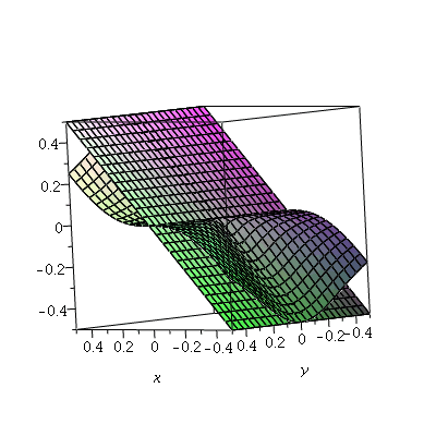
So the "candidate" linear approximating function is  .
But the question is: does that linear function approximate the shape of well 

near  (0,0)? 

>

 

Next, the plot of  

>

 

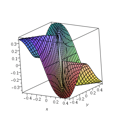What should our conclusion be in this example?  How can we make it rigorous? 

>