MATH 241 -- Multivariable Calculus
Critical Points of Vector Fields
September 28, 2010

Let's consider the vector field  
F(x, y) = (`+`(`*`(2, `*`(`^`(x, 2))), `*`(`^`(y, 3)), `-`(1)), `*`(x, `*`(y)))
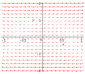
Here is the picture:


with(plots); -1 


fieldplot([`+`(`-`(1), `*`(2, `*`(`^`(x, 2))), `*`(`^`(y, 3))), `*`(x, `*`(y))], x = -1 .. 1, y = -2 .. 2, color = red, fieldstrength = log, arrows = slim); 1 

Plot_2d
 

This vector field has three different critical points -- (0,1), Let's "zoom in" on each one to understand the local picture near each
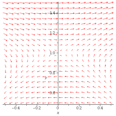
critical point.  First "zoom in" toward (0,1) by changing the ranges of
x-and 

y-values that are plotted: 

fieldplot([`+`(`-`(1), `*`(2, `*`(`^`(x, 2))), `*`(`^`(y, 3))), `*`(x, `*`(y))], x = -.5 .. .5, y = .5 .. 1.5, color = red, fieldstrength = log, arrows = slim); 1
 

Plot_2d
 

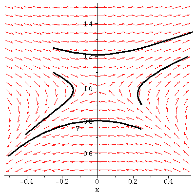
Note that some flow lines here will tend toward the critical point (at least for a while),
while others tend away from it immediately.  Here is a plot showing four flow
 

lines starting from the initial points  (.25,.9), (.25,.75), (-.25,1.1) and (-.25,1.25).
(Note -- we need to use a different command to generate the flow lines!)  
 

with(DEtools); -1 

`assign`(des, [diff(x(t), t) = `+`(`-`(1), `*`(2, `*`(`^`(x(t), 2))), `*`(`^`(y(t), 3))), diff(y(t), t) = `*`(x(t), `*`(y(t)))]); 1 

[diff(x(t), t) = `+`(`-`(1), `*`(2, `*`(`^`(x(t), 2))), `*`(`^`(y(t), 3))), diff(y(t), t) = `*`(x(t), `*`(y(t)))] (1)
 

DEplot(des, [x(t), y(t)], t = 0 .. 2, [[x(0) = .25, y(0) = .9], [x(0) = .25, y(0) = .75], [x(0) = -.25, y(0) = 1.1], [x(0) = -.25, y(0) = 1.25]], x = -.5 .. .5, y = .5 .. 1.5, linecolor = black)
 

Plot_2d
 

This type of critical point is called a saddle point -- it is also said to be unstable, 

since some initial points very close to the critical point give flow lines moving 

away from the critical point. 


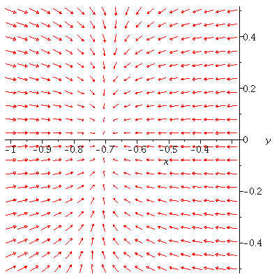
Now we will do the same kind of "zooming in" toward the other critical  

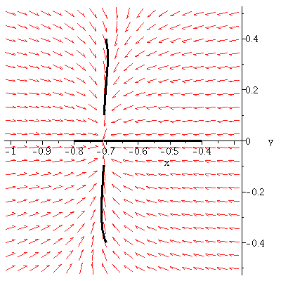
points.  Look at `+`(`-`(`*`(`/`(1, 2), `*`(sqrt(2))))), 0first. 


fieldplot([`+`(`-`(1), `*`(2, `*`(`^`(x, 2))), `*`(`^`(y, 3))), `*`(x, `*`(y))], x = -1 .. -.3, y = -.5 .. .5, color = red, fieldstrength = log, arrows = slim); 1
 

Plot_2d
 

Note that all flow lines starting close to this critical point will tend toward the critical point. 

This type of point is called a sink.  It is said to be stable since flow lines 

that start close to the critical point stay close to it.


DEplot(des, [x(t), y(t)], t = 0 .. 2, [[x(0) = -.7, y(0) = .4], [x(0) = -.7, y(0) = -.4], [x(0) = -.4, y(0) = 0], [x(0) = -.8, y(0) = 0]], x = -1 .. -.3, y = -.5 .. .5, linecolor = black)
 

Plot_2d


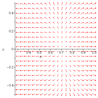
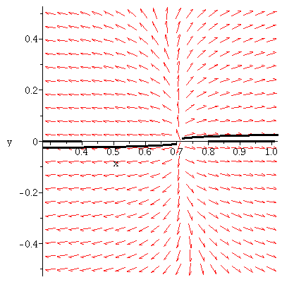
The other critical point at `+`(`*`(`/`(1, 2), `*`(sqrt(2)))), 0looks like this: 

fieldplot([`+`(`-`(1), `*`(2, `*`(`^`(x, 2))), `*`(`^`(y, 3))), `*`(x, `*`(y))], x = .3 .. 1, y = -.5 .. .5, color = red, fieldstrength = log, arrows = slim); 1
 

Plot_2d
 

Note that all flow lines here will tend away from the critical point,


DEplot(des, [x(t), y(t)], t = 0 .. 2, [[x(0) = .717, y(0) = 0.1e-1], [x(0) = .7, y(0) = -0.1e-1], [x(0) = .4, y(0) = 0], [x(0) = .8, y(0) = 0]], x = .3 .. 1, y = -.5 .. .5, linecolor = black)
 

Plot_2d
 

Note that all flow lines starting close to this critical point will tend away from the  

critical point.  This type of point is called a source.  It is said to be unstable  

since flow lines that start close to the critical point move away over time.