MONT 107N -- Understanding Randomness 

``Student's''  t-distributions 

March 29, 2010 

>	read "/home/fac/little/public_html/ProbStat0910/MSP.map":

 

As we have said, there is one  t-curve  for each integer m ≥ 1.   

This integer is called the number of ``degrees of freedom.'' 

(This is one of those cases where there is a reason for the name, 

but it is rather technical.  You might want just to take this as 

a given.  If you are interested, though, I can explain it in 

office hours!) 

The  t-curve with  m  degrees of freedom  is defined by the following 

formula.  (Here the  Γ(x)  is a function generalizing the factorial for 

integers.)   

>	TPDF(m,y);

 

(1)

 

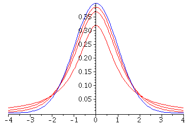
Here are the graphs of several different  t-curves  in red, together with 

the standard normal curve, in blue: 

>	TP:=plot([y->TPDF(1,y),y->TPDF(3,y),y->TPDF(7,y)],-4..4,color=red):

 

>	NP:=plot(y->NormalPDF(0,1,y),-4..4,color=blue):

 

>	with(plots):

 

>	display(TP,NP);

 

We see that the t-curves  have shapes similar to that of the standard 

normal curve,  but with more probability "mass" concentrated in the tails,  

and less concentrated around the average at  0. 

As the number of degrees of freedom   -> ,  though, the  t-curve  

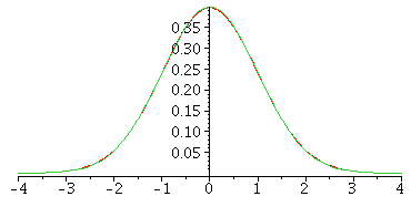
approaches a standard normal normal curve.  Here is the picture 

for  100 degrees of freedom, together with the normal curve 

(note that you cannot easily tell that there are two different curves here!) 

>	plot([y->TPDF(100,y),y->NormalPDF(0,1,y)],-4..4);

 

>