MONT 107N -- Understanding Randomness
Normal and Chi-Square Distributions
April 14, 2010
The first plot shows a histogram for a random sample of size 10000 from a standard
normal distribution. (Note: The scaling is different from what we have used in class, though.
The total area under the normal curve -- in red -- is 1, rather than 100%.)
![]()
![]()
![]()
![]()
 |
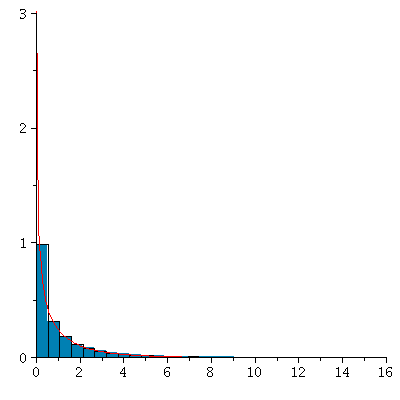
Now we ask, what does the distribution of the squares of the sample values for a sample of size 10000 from
a normally-distributed population look like?
![]()
![]()
![]()
![]()
 |
This is following the curve for a ![]() distribution with one degree of freedom
distribution with one degree of freedom
very closely. This no coincidence. In more mathematical statistics courses,
like the one we teach for math majors, it is proved that the square of a
standard normal random variable has precisely this ![]() distribution(!)
distribution(!)