MONT 105Q -- Mathematical Journeys
Evidence for the Central Limit Theorem -- a family of probability histograms
March 18, 2016
Consider the box [![]() and make
and make ![]() draws with replacement.
draws with replacement.
(This is analogous to choosing a random sample from a large population where
![]() of the individuals are 1's and the other
of the individuals are 1's and the other ![]() are 0's. Note: If the population
are 0's. Note: If the population
is large, then the distinction between sampling with or without replacement
is not too significant.)
Question: What can we say about the distribution of the means of these
samples? How does the size of the sample affect what is going on?
Note that the sum of the draws will equal the number of 1's out of the 35 draws,
so it has a binomial distribution with ![]() and
and ![]() Then the
Then the
mean will equal that number of 1's divided by n.
We will study our question by drawing the probability histograms for the means
of the draws. These will be histograms where the areas of the bars tell us the
probability of getting the corresponding value of the sample mean. What do these
histograms look like as ![]() increases?
increases?
Here is some code (for the computer algebra system Maple we use in
many mathematics courses) in that computes the binomial probabilities
and generates the corresponding probability histograms:
| > |
| > |
| > |
| > |
| > |
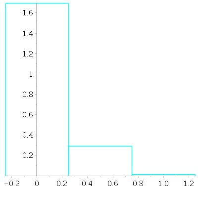
With ![]() draws. Since
draws. Since ![]() is rather small, the probability of a mean of 0 is much larger than the probability
is rather small, the probability of a mean of 0 is much larger than the probability
that the mean is ![]() or
or ![]() The values 0,
The values 0, ![]() are the midpoints of the
are the midpoints of the ![]() intervals at the bases of the boxes. The
intervals at the bases of the boxes. The
heights of the boxes here are normalized so that the total area of the histogram is 1, as we discussed in a problem from
Problem Set 1 earlier.
| > |
 |
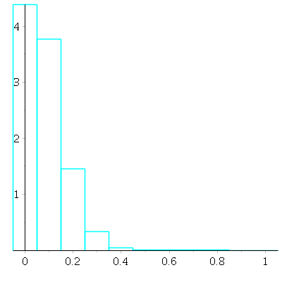
With ![]() draws. Now a mean of 0 is still the likeliest, but a mean of
draws. Now a mean of 0 is still the likeliest, but a mean of ![]() or
or ![]() or
or ![]() is not negligible.
is not negligible.
| > |
 |
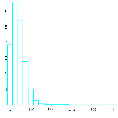
With ![]() draws -- now the likeliest mean is not zero any more(!)
draws -- now the likeliest mean is not zero any more(!)
| > |
 |
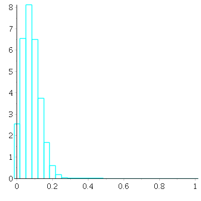
With ![]() draws. At this point, notice that the probability histogram is starting to look more "normal" in shape(!)
draws. At this point, notice that the probability histogram is starting to look more "normal" in shape(!)
| > |
 |
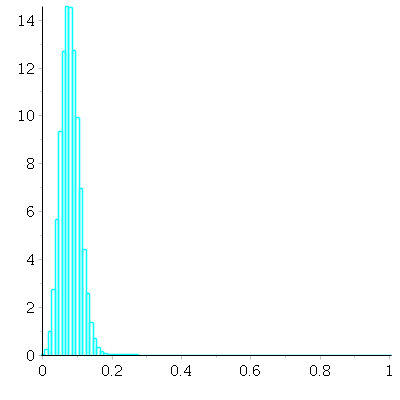
Finally, with ![]() draws:
draws:
| > |
 |
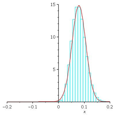
Now we find an approximating normal curve to this probability histogram. The mean is ![]() = average
= average
of original box. The SD is the SD of the box multiplied by the reciprocal of the square root of the
sample size: ![]() We define that shifted, scaled normal curve, and plot it in red
We define that shifted, scaled normal curve, and plot it in red
together with the N = 100 probability histogram to see how closely it matches:
| > |
| > |
| > |
| > |
 |
| > |