MATH 132 -- Calculus for Physical and Life Sciences 2  

Lab 3 -- Logistic Models with Harvesting (Environmental Modeling) 

April 7, 2008 

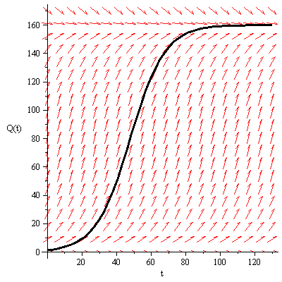
Question A:  The logistic equation and the solution with  Q(0) = 1.3 Mg 

(1)

 

A 2)  The formula for the solution of the logistic equation is:
 

(2)

 

(3)

 

(4)

 

These are the biomass values at the times t = 0, 10, 20, ... , 150 years:

 

(5)

 

A 3)  The recovery time is the time it takes the forest to regrow to 99% of the carrying capacity, or (.99)(160) = 158.4: 

(6)

 

Thus the recovery time is about 94 years. 

B)  
 

1)  The "virgin state" would be represented by the initial value Q(0) = 160.

2 and 3)  With 3.2 Mg of biomass harvested each year, the differential equation becomes:

 

(7)

 

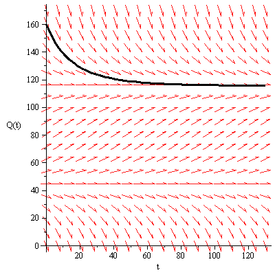4) Note that the solution seems to be tending to a limiting value of about Q = 116 as  
5)  With the harvesting level at 6.4 Mg/year, the differential equation becomes 

(8)

 

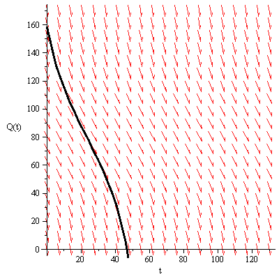The solution reaches the value Q = 0 at about t = 47 years.  At that time, all the biomass in the forest 

has been removed.  

C)  To find the equilibria of these differential equations with the harvesting terms, we need to  

set the right-hand sides equal to zero and solve for Q.  This can be done in Maple as follows. 

For the harvesting level of 3.2 Mg/year, we use: 

>

 

(9)

 

in the plot of the solutions for the equation with the harvesting 

level of 3.2 Mg/year above.   The solutions tend toward the 115.78 level, they tend away from the 44.22 

level.  These values can also be derived by using the quadratic formula to solve this quadratic equation 

for Q:    

>	(-.1 + sqrt((.1)^2 - 4*(-1/1600)*(-3.2)))/(2*(-1/1600));

 

(10)

 

>

 

(11)

 

On the other hand, with the harvesting term 6.4 Mg/year, the quadratic equation  

(12)

 

has no real roots, so there are no equilibria. 

D)  With selective harvesting strategy 1, the biomass level is tending to 115.78 Mg in the long run, 

      so 3.2 Mg can be harvested every year, and the average yield per year is 3.2 Mg/year. 

     With the clear-cutting strategy (after the first cycle), we would be taking 158.4 - 1.3 Mg 

     then letting the forest regrow for 94 years, so the average yield per year is  

     Mg/year.

     With the selective harvesting strategy 2, there are 6.4 Mg harvested in the first 47 or so years, 

     then the forest is allowed to regrow for 94 years with no harvesting, then the cycle repeats.  This gives  

     an average yield per year of  Mg/year.

E)  
     1)  The maximum sustainable harvesting level is exactly 4.0 Mg/year (per hectare).  This can be seen 

          algebraically, since the largest value of   h  for which the quadratic equation  

     has real roots is when  so h = 4.
 

      2) Note that the question is asking if it is possible to tell a forest that is undergoing a sustainable 

          harvesting strategy apart from a "virgin" forest.  It's true that there are logging operations 

          going on, so the forest is not undisturbed, but the deeper question is:  Can we tell something 

          measurable that is different?  The best answer here is that the sustainable equilibrium level  

          of the biomass decreases with harvesting, so the forest is qualitatively different (it would be  

          less "thick" or "dense" forest).  This can be seen by comparing the sustainable equilibrium  

          of 115.78 Mg (per hectare) from Strategy 1 with the "virgin" level of  160 Mg/hectare.  It's  

          not the same forest with harvesting! 

    3)  (No one really saw the point of this one, so I gave everyone 4 free points here)  What this 

         question was getting at was to compare Strategies 1 and 2.  From question D, the average 

         yield per hectare per year with Strategy 1 was larger  than with Strategy 2 even though the  

         harvesting level was smaller with Strategy 1 as compared with Strategy 2.   If the forest 

         had enough area so that the loggers would have something to do every year on part of the  

         forest while other parts were regrowing, then the lower annual harvest level actually could  

         keep people employed and produce higher average yields.