>

 

MATH 131, section 1 -- Calculus for Physical and Life Sciences 1 

"Advanced Graphing" with Calculus and Calculators/Maple 

November 12, 2007. 

First, let's take a fairly complicated rational function like 

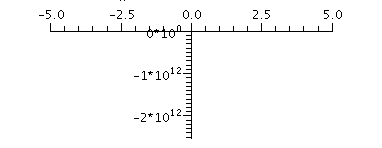
Let's see what happens if we plot this "blindly": 

>

 

>

 

Pretty uninformative, right!   What is going on here?  It should be 

somewhat clear from the formula that the graph has vertical asymptotes  

that are producing the huge range of  y - values shown in this plot. 

We can also analyze the function to see which direction the graph 

should be approaching the asymptotes.  The results of this are that 

the graph should be going down to on both sides of 0.  It should 

be tending to as and it should be tending to as  

Moreover,  

so the x-axis is a horizontal asymptote. 

  We should begin by cutting down the y-range (and also tell Maple to  

expect discontinuities) to get something more reasonable: 

>

 

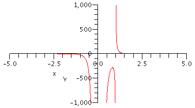
This is a lot closer to an accurate plot of the function. 

Note in particular that it seems that there is a local  

maximum on the part of the graph on the interval 

(0,1)  which matches what we said above about the  

direction of approach to the asymptotes! 

But we are still missing some important features of this  

function(!)   Note that  

from the factorization of the numerator.  So in fact the graph should 

intersect the x-axis at x = -4  and again at x = 3.  This is  

not clear at all from the plot above.  And there's no way we're ever 

going to see those intersections with a range of y-values that  

is this big (-1000 ≤ y ≤ 1000).  

So in fact to see what is going on, we should probably not look just at  

one graph, but rather look at separate plots for x  around 

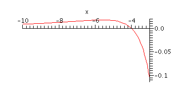
-4  and for x  around 3.   Here's a plot for  -10 ≤ x ≤ -3 

which shows that the graph crosses from positive to negative 

y-values at  

>

 

>

 

Note that this forces a local maximum of  f  somewhere to the left of  

apparently around so, since  f  is tending to  0  as 

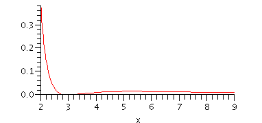
Let's also plot  f  on a range of values starting to the left of 3 

and going past 3 to the right.   

>

 

Notice that the graph appears to be tangent to the x-axis at  

Since  f  tends to 0 as  this means that there 

must be another local maximum somewhere to the right of  

This is apparently at about although it is difficult  

to tell since the graph seems very flat between 5 and 6).   

So at this point we can see from the plots: 

  ▽ f   has vertical asymptotes at  

  ▽ f  has a horizontal asymptote at  

  ▽ f  has at least 4 critical numbers  (where  

Are we missing any other important features (e.g. other 

critical numbers, etc.?   

Sophisticated programs like Maple can be used to  

compute derivatives as well as generate graphs.  Here's 

the derivative of our function, simplified: 

>

 

The critical numbers are the roots of the numerator.  Maple 

also has numerical routines for finding approximate solutions 

of equations:  

>

 

Since there are only 4 roots (including all the critical numbers found 

above), this is apparently a complete picture now! 

>