MATH 131 -- Calculus for Physical and Life Sciences 1

Lab 4 -- Families of Curves, solutions

November 23, 2004

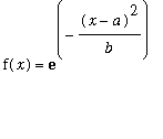
A)  The family  

1)  

>	f:=(x,a,b)->exp(-(x-a)^2/b);

>	plot([f(x,0,.1),f(x,0,1),f(x,0,3),f(x,0,10)],x=-10..10,color=[blue,green,red,black]);

Varying   b   keeping   a   fixed ``stretches'' the graph horizontally as   b   increases.  The

widest curve here is the curve for   b = 10.

2)

>	plot([f(x,-2,1),f(x,-1,1),f(x,0,1),f(x,1,1),f(x,2,1)],x=-4..4,color=[blue,green,red,black,gray]);

Varying   a   while keeping   b   fixed shifts the graph left (if a < 0 ) or right (if a > 0 ).

3)  The critical points come from solutions of   f '(x)  = 0:

>	solve(diff(f(x,a,b),x)=0,x);

Each curve in the family has exactly one critical point, at   x = a.   The critical

  point is always a local maximum -- that doesn't change with different values

of   a, b.   To see this, here is the plot of   f '   for the curve in the family with

a = 0,  b = 1.   By the First Derivative Test,  f  has a local maximum    x = 0

because   f ' changes from positive to negative at the critical point:

>	plot(diff(f(x,0,1),x),x=-2..2);

This does match the plots above.

4)  Inflection points come from solutions of   f '' (x) = 0

>	solve(diff(diff(f(x,a,b),x),x)=0,x);

Each curve in the family has exactly two inflection points, one to the left of the

maximum, one to the right.

B)  The family  

1)

>	g:=(x,a)->x^3 - 3*a*x + 1;

>	plot([g(x,-2),g(x,-1),g(x,0),g(x,1),g(x,2)],x=-3..3,color=[blue,green,red,black,gray]);

>	diff(g(x,a),x);

2)  The curves in this family have two critical points   ,     if

a > 0, one critical point at   x = 0 if   a = 0, and no critical points if   a < 0.

3)  The curve in the family with a double root is the one where  

so the graph is tangent to the x -axis at the critical point.  

>	solve(g(sqrt(a),a)=0,a);

>	plot(g(x,2^(1/3)/2),x=-3..3);

C)  The family  

>	h:=(x,a,b)->1/((x-a)^2+b);

1)  Fixing a, varying b

>	plot([h(x,0,-2),h(x,0,-1),h(x,0,-.2),h(x,0,.2),h(x,0,1),h(x,0,2)],x=-3..3,y=-10..10,discont=true);

2)  Fixing  b=-1,  varying   a:

>	plot([h(x,-2,-1),h(x,-1,-1),h(x,0,-1),h(x,1,-1),h(x,0,1)],x=-3..3,y=-10..10,discont=true);

3)  The graph of   h   has vertical asymptotes where   .  This equation

can be solved for   x   only when   b <= 0.   The locations of the asymptotes are  

x = a +   and  

4)  

>	solve(diff(h(x,a,b),x)=0,x);

There is one critical point in each case, and it is a local maximum.

5)  To get a local maximum at  (3,5),  we want a = 3   by the above.

Then to get   y = 5,     implies   b = .2

>	plot(h(x,3,.2),x=1..5);

6)

>	solve(diff(diff(h(x,a,b),x),x)=0,x);

The curves in the family have two inflection points for all b > 0   (but none if b < 0).

These are visible in the plot from part 5 above.