MATH 132 -- Calculus for Physical and Life Science 2
Solutions for Lab Day 1 -- "In Search of a Better Numerical
Integration Method"
A) 1) First integral:
| > | with(student); |
![]()
![]()
| > | f1:=exp(-x^2/10); |
| > | exact1:=evalf(Int(f1,x=0..2)); |
![]()
| > | n:='n'; |
![]()
| > | with(Spread): |
| > | Table1:=CreateSpreadsheet(): |
![]()
| > | ns:=[5,10,20,40,80,160]; |
![]()
| > | for i to 6 do SetCellFormula(Table1,i+1,1,ns[i]); SetCellFormula(Table1,i+1,2,evalf(leftsum(f,x=0..2,ns[i]))); SetCellFormula(Table1,i+1,3,evalf(middlesum(f,x=0..2,ns[i]))); SetCellFormula(Table1,i+1,4,evalf(rightsum(f,x=0..2,ns[i]))); SetCellFormula(Table1,i+1,5,evalf(trapezoid(f,x=0..2,ns[i]))); SetCellFormula(Table1,i+1,6,exact1-evalf(leftsum(f,x=0..2,ns[i]))); SetCellFormula(Table1,i+1,7,exact1-evalf(middlesum(f,x=0..2,ns[i]))); SetCellFormula(Table1,i+1,8,exact1-evalf(rightsum(f,x=0..2,ns[i]))); SetCellFormula(Table1,i+1,9,exact1-evalf(trapezoid(f,x=0..2,ns[i]))); |
| > | end do; |
| > | EvaluateSpreadSheet(Table1); |
![]()
| > |
2) Second integral:
| > | f2:=sin(x)/x; |
![]()
| > | Table2:=CreateSpreadsheet(); |
![]()
| > |
| > | ns:=[5,10,20,40,80,160]; |
![]()
| > | exact2:=evalf(Int(f2,x=2..5)); |
![]()
| > | for i to 6 do SetCellFormula(Table2,i+1,1,ns[i]); SetCellFormula(Table2,i+1,2,evalf(leftsum(f2,x=2..5,ns[i]))); SetCellFormula(Table2,i+1,3,evalf(middlesum(f2,x=2..5,ns[i]))); SetCellFormula(Table2,i+1,4,evalf(rightsum(f2,x=2..5,ns[i]))); SetCellFormula(Table2,i+1,5,evalf(trapezoid(f2,x=2..5,ns[i]))); SetCellFormula(Table2,i+1,6,exact2-evalf(leftsum(f2,x=2..5,ns[i]))); SetCellFormula(Table2,i+1,7,exact2-evalf(middlesum(f2,x=2..5,ns[i]))); SetCellFormula(Table2,i+1,8,exact2-evalf(rightsum(f2,x=2..5,ns[i]))); SetCellFormula(Table2,i+1,9,exact2-evalf(trapezoid(f2,x=2..5,ns[i]))); |
| > | end do; |
| > | EvaluateSpreadSheet(Table2); |
![]()
3) Third Integral:
![]()
| > | ns:=[5,10,20,40,80,160]; |
![]()
| > | f3:=sqrt(1+x^4); |
![]()
| > | exact3:=evalf(Int(f3,x=0..1)); |
![]()
| > | Table3:=CreateSpreadsheet();
|
![]()
| > | for i to 6 do SetCellFormula(Table3,i+1,1,ns[i]); SetCellFormula(Table3,i+1,2,evalf(leftsum(f3,x=0..1,ns[i]))); SetCellFormula(Table3,i+1,3,evalf(middlesum(f3,x=0..1,ns[i]))); SetCellFormula(Table3,i+1,4,evalf(rightsum(f3,x=0..1,ns[i]))); SetCellFormula(Table3,i+1,5,evalf(trapezoid(f3,x=0..1,ns[i]))); SetCellFormula(Table3,i+1,6,exact3-evalf(leftsum(f3,x=0..1,ns[i]))); SetCellFormula(Table3,i+1,7,exact3-evalf(middlesum(f3,x=0..1,ns[i]))); SetCellFormula(Table3,i+1,8,exact3-evalf(rightsum(f3,x=0..1,ns[i]))); SetCellFormula(Table3,i+1,9,exact3-evalf(trapezoid(f3,x=0..1,ns[i]))); |
| > | end do; |
| > | EvaluateSpreadSheet(Table3); |
![]()
B) 1) You might notice that the error decreases when we double n in every case. Moreover, the
size of the error seems to decrease roughly by a factor of 2 when we double n for the
LEFT and RIGHT methods, and roughly by a factor of 4 when we double n for the
MID and TRAP methods.
2) When we fix n the LEFT and RIGHT errors are usually close to each other in magnitude, and
also usually quite a bit larger than the MID and TRAP errors. Also, when we compare
the MID and TRAP errors, we see that they have opposite signs, and the TRAP error is
roughly twice as large in magnitude.
3) The MID method gives an overestimate (negative error) if the graph is concave down
and an underestimate (positive error) if the graph is concave up. We have the first
case in integral 1, and the second for integrals 2 and 3
C) 1) Using Simpson's Rule
.
| > | Table4:=CreateSpreadsheet()
|
![]()
| > | for i from 2 to 6 do SetCellFormula(Table4,i,1,ns[i]); SetCellFormula(Table4,i,2,evalf(simpson(f1,x=0..2,ns[i]))); SetCellFormula(Table4,i,4,evalf(simpson(f2,x=2..5,ns[i]))); SetCellFormula(Table4,i,6,evalf(simpson(f3,x=0..1,ns[i]))); SetCellFormula(Table4,i,3,exact1-evalf(simpson(f1,x=0..2,ns[i]))); SetCellFormula(Table4,i,5,exact2-evalf(simpson(f2,x=2..5,ns[i]))); SetCellFormula(Table4,i,7,exact3-evalf(simpson(f3,x=0..1,ns[i]))); end do; |
Note that the errors here are all significantly smaller than the corresponding errors for
LEFT, RIGHT, and even MID and TRAP.
2) The reason that the SIMPSON method is significantly more accurate is the relationship
between the MID and TRAP errors we noted in B 3. Recall that we said that the TRAP
error was roughly twice as large in magnitude, and of the opposite sign than the
MID error. This means when we form the weighted average:
SIMPSON(n) =
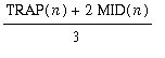
the errors are almost cancelling out. (They would exactly cancel out and yield an error
of zero if the TRAP error was exactly twice as large as the MID error in magnitude).