| > |
| > |
MATH 244 -- Linear Algebra Section 1
Problem Set 9 Solutions
April 20, 2007
Section 5.2
6. The characteristic polynomial is 
The eigenvalues are the roots of 0 = ![]() so by the quadratic
so by the quadratic
formula:
![]()
![]()
![]()
Neither root is real, so there are no real eigenvalues.
10. The characteristic polynomial is
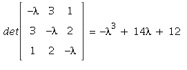 (after expanding out and simplifying).
14. The characteristic polynomial is (expanding determinant along row 2):

![]()
18. The eigenspace for ![]() is:
is:
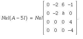 If we consider reducing this to row-reduced
echelon form, then there is only one free variable in the system ![]()
unless ![]() For h = 6, we have rref =
For h = 6, we have rref = 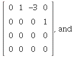
![]()
, Vector[column](%id = 138526992)})](images/PS9Sol_16.gif) dimension 2. In all other cases
dimension 2. In all other cases ![]()
23. If ![]() then
then  This shows that
 ![]() and
and
![]() are similar since the invertible matrix
are similar since the invertible matrix ![]() satisfies
satisfies ![]()
(see the definition at bottom of page 314 in the text).
25. a) By direct calculation, ) = Vector[column](%id = 136084140) and Vector[column](%id = 136084140) = Vector[column](%id = 140169988)](images/PS9Sol_24.gif)
so the given vector is an eigenvector with eigenvalue λ = 1. The characteristic
polynomial is ![]() so the other eigenvalue is
so the other eigenvalue is
 Since the eigenvalues
1 and .3 are distinct, the set , Vector[column](%id = 135143236)}](images/PS9Sol_27.gif) is linearly independent (Theorem 2 on
is linearly independent (Theorem 2 on
page 307 of the text, or direct check), hence a basis for ![]()
b) ![]()
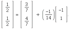
c) This is similar to the computations you did on Discussion 3:
![x[1] = Ax[0] and Ax[0] = (Matrix(%id = 140198924))(Vector[column](%id = 139342576)+`.`(-1/14, Vector[column](%id = 138411204))) and (Matrix(%id = 140198924))(Vector[column](%id = 139342576)+`.`(-1/14,...](images/PS9Sol_31.gif)
![]()
![x[2] = Ax[1] and Ax[1] = (Matrix(%id = 136393492))(Vector[column](%id = 136328928)+`.`((-1/14)(.3), Vector[column](%id = 135967588))) and (Matrix(%id = 136393492))(Vector[column](%id = 136328928)+`.`(...](images/PS9Sol_33.gif)
![x[2] = Ax[1] and Ax[1] = (Matrix(%id = 136393492))(Vector[column](%id = 136328928)+`.`((-1/14)(.3), Vector[column](%id = 135967588))) and (Matrix(%id = 136393492))(Vector[column](%id = 136328928)+`.`(...](images/PS9Sol_34.gif)
Similarly, for all ![]() , by mathematical induction,
, by mathematical induction,
![]()


In the limit as  so
so 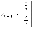
Section 5.3
12. Given that the eigenvalues are ![]() we have
we have


Then, ℬ = , Vector[column](%id = 138003488), Vector[column](%id = 140090712)}](images/PS9Sol_44.gif) is a basis for
is a basis for ![]() consisting of eigenvectors
consisting of eigenvectors
of A. This shows that A is diagonalizable, with  for
for
 Check:
| > |
![table( [( 3, 3 ) = 8, ( 2, 2 ) = 2, ( 3, 2 ) = 0, ( 2, 1 ) = 0, ( 3, 1 ) = 0, ( 2, 3 ) = 0, ( 1, 2 ) = 0, ( 1, 3 ) = 0, ( 1, 1 ) = 2 ] )](images/PS9Sol_51.gif)
14. Given the eigenvalues are ![]() (characteristic polynomial factors as
(characteristic polynomial factors as
![]() Theorem 7 on page 326 implies that in order for
Theorem 7 on page 326 implies that in order for
A to be diagonalizable, we must have ![]()
 which is row-equivalent to
  so there are 2 free
variables in the homogeneous system ![]()
 Then
Then 
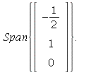 This shows that A is diagonalizable with
| > |
![table( [( 3, 3 ) = 0, ( 2, 2 ) = 0, ( 3, 2 ) = 1, ( 2, 1 ) = 1, ( 3, 1 ) = 0, ( 2, 3 ) = 1, ( 1, 2 ) = -2, ( 1, 3 ) = -1/2, ( 1, 1 ) = 0 ] )](images/PS9Sol_63.gif)
| > |
![table( [( 3, 3 ) = 5, ( 2, 2 ) = 5, ( 3, 2 ) = 0, ( 2, 1 ) = 2, ( 3, 1 ) = 0, ( 2, 3 ) = 4, ( 1, 2 ) = 0, ( 1, 3 ) = -2, ( 1, 1 ) = 4 ] )](images/PS9Sol_65.gif)
| > |
![table( [( 3, 3 ) = 4, ( 2, 2 ) = 5, ( 3, 2 ) = 0, ( 2, 1 ) = 0, ( 3, 1 ) = 0, ( 2, 3 ) = 0, ( 1, 2 ) = 0, ( 1, 3 ) = 0, ( 1, 1 ) = 5 ] )](images/PS9Sol_67.gif)
24. No -- the hypotheses of Theorem 7 on page 324 cannot be satisfied in
this case. The largest linearly independent set of eigenvectors will have
size 2, so there is no basis consisting of ![]() consisting of eigenvectors of A.
consisting of eigenvectors of A.
26. Yes -- if the remaining eigenspace has dimension only 1, then the matrix
is not diagonalizable (see Theorem7). The following matrix gives an example
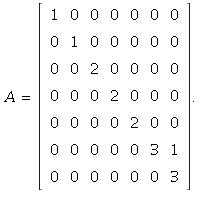 The eigenvalues are
 ![]() (with multiplicity 2),
(with multiplicity 2),
![]() with multiplicity 3) , and
with multiplicity 3) , and ![]() (with multiplicity 2). By the form of the
(with multiplicity 2). By the form of the
matrix ![]() has dimension 2,
has dimension 2, ![]()
has dimension 3, but ![]()
32. Since A is not invertible, ![]() must be one of the eigenvalues (see Theorem on page
must be one of the eigenvalues (see Theorem on page
312 -- continuation of the Invertible Matrix Theorem). By Theorem 6 on page 323,
if the other eigenvalue is ![]() (or anything other than 0), then A will be diagonalizable.
(or anything other than 0), then A will be diagonalizable.
This means that A should be similar to the diagonal matrix  To get
![]() not diagonal we can try taking an arbitrary invertible matrix like
not diagonal we can try taking an arbitrary invertible matrix like  with
with
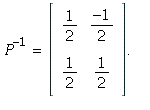 Then
Then ![]()
| > |
![table( [( 2, 2 ) = 1/2, ( 2, 1 ) = -1/2, ( 1, 2 ) = -1/2, ( 1, 1 ) = 1/2 ] )](images/PS9Sol_85.gif)
is a matrix that satisfies all of the properties we want.
Section 6.2
6. Call the three vectors ![]() We have
We have
![]()
![]()
![]()
So the set is not orthogonal. (It would be enough just to show ![]()
of course).
10. It is clear that ![]() here. This implies that
here. This implies that
![]() is an orthogonal set. By Theorem 4 in this section, it
is an orthogonal set. By Theorem 4 in this section, it
follows that ![]() is linearly independent. (This can also be checked
is linearly independent. (This can also be checked
directly: If ![]() for some scalars
for some scalars ![]() then
then
we can take dot products with ![]()
0 = ![]()
Since ![]() Similarly, dotting with
Similarly, dotting with ![]() shows
shows ![]() and
and
dotting with ![]() shows
shows ![]() It follows that
It follows that![]() is a basis for
is a basis for ![]()
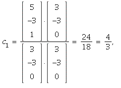
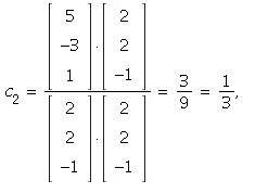
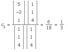
Then because of the orthogonality, there is a shortcut we can use for
computing the weights in a linear combination:
![]()
For each i, i = 1, 2, 3, we have
![]() (since the dot product of
(since the dot product of ![]() with the other two terms
with the other two terms
is zero).
Hence ![c[i] = x*u[i]/`*`(u[i], u[i])](images/PS9Sol_108.gif) for each i = 1, 2, 3.
for each i = 1, 2, 3.
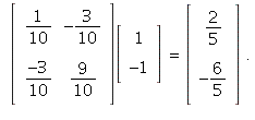
12. The orthogonal projection on the line spanned by ](images/PS9Sol_112.gif) is defined by
is defined by


With  we get
| > |
![]()
| > |
![table( [( 3, 3 ) = 8, ( 2, 2 ) = 2, ( 3, 2 ) = 0, ( 2, 1 ) = 0, ( 3, 1 ) = 0, ( 2, 3 ) = 0, ( 1, 2 ) = 0, ( 1, 3 ) = 0, ( 1, 1 ) = 2 ] )](images/PS9Sol_122.gif)
| > |