| > |
MATH 244 -- Linear Algebra
Problem Set 3 Solutions
February 9, 2007
1.8/4. Since ![]() , this question is asking
, this question is asking
whether the system ![]() has any solutions, and
has any solutions, and
if so, whether the solution is unique.
| > |
![table( [( 3, 4 ) = -9, ( 1, 3 ) = 2, ( 1, 4 ) = 6, ( 2, 3 ) = -4, ( 1, 2 ) = -3, ( 2, 1 ) = 0, ( 3, 1 ) = 3, ( 2, 4 ) = -7, ( 3, 3 ) = -9, ( 1, 1 ) = 1, ( 3, 2 ) = -5, ( 2, 2 ) = 1 ] )](images/PS3Sol_5.gif)
| > |
![table( [( 3, 4 ) = 1, ( 1, 3 ) = 0, ( 1, 4 ) = -5, ( 2, 3 ) = 0, ( 1, 2 ) = 0, ( 2, 1 ) = 0, ( 3, 1 ) = 0, ( 2, 4 ) = -3, ( 3, 3 ) = 1, ( 1, 1 ) = 1, ( 3, 2 ) = 0, ( 2, 2 ) = 1 ] )](images/PS3Sol_7.gif)
Since the rref has a pivot in each row of A, there is a unique x =
](images/PS3Sol_8.gif)
1.8/5 Same idea as number 4 above:
| > |
![table( [( 1, 3 ) = -7, ( 1, 4 ) = -2, ( 2, 3 ) = 5, ( 1, 2 ) = -5, ( 2, 1 ) = -3, ( 2, 4 ) = -2, ( 1, 1 ) = 1, ( 2, 2 ) = 7 ] )](images/PS3Sol_10.gif)
| > |
![table( [( 1, 3 ) = 3, ( 1, 4 ) = 3, ( 2, 3 ) = 2, ( 1, 2 ) = 0, ( 2, 1 ) = 0, ( 2, 4 ) = 1, ( 1, 1 ) = 1, ( 2, 2 ) = 1 ] )](images/PS3Sol_12.gif)
The system is consistent, but there is a free variable so the
solution is not unique. The general solution looks like
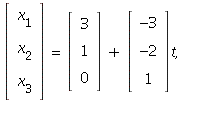 where
where ![]() is arbitrary.
is arbitrary.
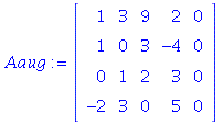
1.8/10. This question asks for all the solutions of the
homogeneous system ![]()
| > |
| > |
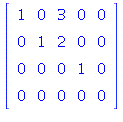
Because of the row of zeroes, this system has a free variable (![]() . The
. The
solutions can be parametrized as:
 = `.`(Vector[column](%id = 135143236), t)](images/PS3Sol_21.gif) where
where ![]() is arbitrary.
is arbitrary.
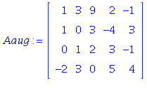
1.8/12. Now we consider the same coefficient matrix as in 10, but
the question is whether Ax = b has solutions for b ≠ 0.
| > |
| > |
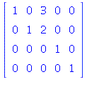
The inhomogeneous system is inconsistent (look at the last row).
Hence b is not in the range of this linear transformation.
1.8/19. We are given that ![T(e[1]) = y[1] and y[1] = Vector[column](%id = 138386324)](images/PS3Sol_27.gif) and
and 
Hence the standard matrix of T is A = Then,
Then,

 If
If 


1.8/27
a) The usual parametrization of the line through p and q uses
the direction vector v = q - p, and the points on the line
are x = p + t(q - p), for all ![]() This can be rearranged
This can be rearranged
using the distributive law for scalar multiplication over vector
sums: x = (![]() p + tq. The line segment from p to q is
p + tq. The line segment from p to q is
the portion of the line with ![]()
b) If T is a linear transformation then applying T to the points
on the line segment from part a and using the definition of
linearity yields:
![]() (
(![]() p + tq) = T((1 - t)p) + T(tq)
p + tq) = T((1 - t)p) + T(tq)
= (1 - t) T(p) + t T(q)
When ![]() we have the points on the line segment
we have the points on the line segment
from T(p) to T(q) (note the final equation here looks
just like the parametrization of the line segment from
p to q in the domain of the mapping, but it gives points
in ![]() )
)
If T(p) ≠ T(q), then we have an actual line segment.
If T(p) = T(q), though, then we get the same point for
all ![]() the line segment is collapsed to a point by
the line segment is collapsed to a point by
T).
1.8/28 The idea is similar to number 27. The points in
the parallelogram spanned by u, v are the au + bv,
where 0 ≤ a ≤ 1 and ![]() If we apply T to any
If we apply T to any
one of these points, using the properties in the definition
of linearity, we get
![]() T( au + bv) = T(au) + T(bv)
T( au + bv) = T(au) + T(bv)
= a T(u) + b T(v)
This gives one of the points in the parallelogram spanned
by T(u) and T(v) (if it's actually a parallelogram). Comment:
As in the previous problem there are also "special cases"
depending on the mapping and the actual vectors. In
some cases, the parallelogram could be mapped onto a
line segment (if T(u) and T(v) are collinear), or a single
point (if T(u) and T(v) are both 0).
1.9/2 By the definition of the standard matrix of T, we
put T(![]() ) in the first column T(
) in the first column T(![]() ) in the second
) in the second
column and T(![]() ) in the third:
) in the third:

1.9/4. The process is the same is in 2 above, but
now the matrix will be 2 x 2 since we the domain is
![]() The vectors T(
The vectors T(![]() ) and T(
) and T(![]() ) are found by
) are found by
trigonometry -- in an isosceles right triangle with
hypotenuse of length 1, the legs have length ![]()
Since we rotate by π/4 clockwise, T(![]() ) is
) is
in the 4th quadrant (x > 0, y < 0) and T(![]() ) is in the
) is in the
first quadrant.
So A = 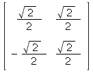
1.9/6. Using the description given in the problem,

1.9/8. Applying the two steps making up T in succession,
we get
![]()
![]()
so 
(Comment: This is the same transformation
as a counter-clockwise rotation through an angle of π/2
about the origin(!))
1.9/31. "T is one-to-one if and only if A has
n pivot columns." (Note: This means every column
in A is a pivot column, because A has n
columns all together).
This is true because T is one-to-one if and only
if the homogeneous system A x = 0 has only the
trivial solution (Theorem 11). T is one-to-one
if and only if there are no free variables in the
homogeneous system.
1.9/32. "T maps ![]()
![]() onto
onto ![]() if and only if A
if and only if A
has m pivot columns." This is true because saying
T is onto is the same as saying A x = b is
consistent for all ![]() equivalently,
equivalently,
that the columns of A span ![]() This means that
This means that
every row must have a pivot, so there are m
columns containing pivots. (Theorem 12)
1.9/35. If T is one-to-one then ![]()
If T is onto, then ![]() These assertions
These assertions
follow from problems 31 and 32 above, since
the matrix of T is n x m.
1.9/36. For all x, y ![]() and scalars c we have
and scalars c we have
T( S ( x + y )) = T ( S (x) + S (y) ) (since S is linear)
= T ( S (x) ) + T ( S (y) ) (since T is linear)
and
T( S ( c x ) ) = T( c S ( x ) ) (since S is linear)
= c T( S ( x ) ) (since T is linear)
Since the composite mapping satisfies the two properties
in the definition, it is also linear.
2.2/3.
We can follow the process described in class:
| > |
![table( [( 1, 3 ) = 1, ( 1, 4 ) = 0, ( 2, 3 ) = 0, ( 1, 2 ) = 5, ( 2, 1 ) = -7, ( 2, 4 ) = 1, ( 1, 1 ) = 8, ( 2, 2 ) = -5 ] )](images/PS3Sol_69.gif)
| > |
![table( [( 1, 3 ) = 1, ( 1, 4 ) = 1, ( 2, 3 ) = -7/5, ( 1, 2 ) = 0, ( 2, 1 ) = 0, ( 2, 4 ) = -8/5, ( 1, 1 ) = 1, ( 2, 2 ) = 1 ] )](images/PS3Sol_71.gif)
Then the inverse is the right-hand 2 x 2 block
| > |
![table( [( 1, 2 ) = 1, ( 2, 1 ) = -7/5, ( 1, 1 ) = 1, ( 2, 2 ) = -8/5 ] )](images/PS3Sol_73.gif)
2.2/6 When A is invertible, A x = b has a unique
solution for all b. The solution is x = ![]()
| > |
![table( [( 2, 1 ) = -5, ( 1, 1 ) = 2 ] )](images/PS3Sol_76.gif)
2.2/15. The matrix ![]()
2.2/18. To solve ![]() for B, we have to realize
for B, we have to realize
that matrix multiplication is not commutative. This means,
for instance, that if we multiply both sides of the equation
by P to cancel the ![]() on the right of B, then that P
on the right of B, then that P
must go on the right on both sides of the equation.
![]()
![]()
![]()
Hence ![]()
2.2/19. Proceed as in 18:
![]()
Multiply both sides of the equation by ![]() and
and ![]()
(and group terms by associativity)
![((1/CC)(A+X))(`*`(1/B, B)) = CI[n]*B and CI[n]*B = CB](images/PS3Sol_87.gif)
![]()
![]()
2.2/31
| > |

| > |
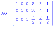
| > |
![table( [( 1, 3 ) = 1, ( 2, 3 ) = 1, ( 1, 2 ) = 3, ( 2, 1 ) = 10, ( 3, 1 ) = 7/2, ( 3, 2 ) = 3/2, ( 3, 3 ) = 1/2, ( 1, 1 ) = 8, ( 2, 2 ) = 4 ] )](images/PS3Sol_95.gif)
2.2/32
| > |

| > |
![table( [( 1, 3 ) = 0, ( 2, 3 ) = 0, ( 1, 2 ) = 0, ( 2, 1 ) = -1, ( 3, 1 ) = 0, ( 3, 2 ) = -1, ( 3, 3 ) = 1, ( 1, 1 ) = 1, ( 2, 2 ) = 1 ] )](images/PS3Sol_99.gif)
| > |
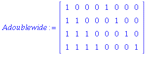
| > |
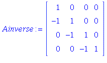
From these examples, you should conjecture that the
inverse of the general matrix A of this form is the
matrix B with 1 on the main diagonal, -1 on
the subdiagonal, and zeroes everywhere else.
There are many ways to show that AB = BA = ![]() for
for
general n . The most direct way is probably to notice
that when you multiply B of this form on the left of
any matrix, you are performing a sequence of row
operations on that matrix:
* ![]() is unchanged,
is unchanged,
* ![]()
* ![]()
...
* ![]()
Whe you perform these row operations on the matrix A,
for each i > 1, the i th row of A contains 1's in columns
1, 2, ... i, while the (i - 1)st row contains 1's in columns
1,2, ..., i-1. The row operation ![]()
the first i - 1 1's and leaves the 1 in row i and column i .
Hence the product BA is the matrix ![]()
It actually follows that AB = ![]() too by the Invertible
too by the Invertible
Matrix Theorem. However, we can also prove this as follows.
Similarly to what we said above about multiplying by B,
when you multiply A on the left of any matrix,
you are also doing a sequence of row operations:
* ![]() is unchanged
is unchanged
* ![]()
* ![]() (two operations)
(two operations)
...
* ![]() (i-1 operations in all)
(i-1 operations in all)
...
* ![]() n-1 operations in all)
n-1 operations in all)
When you apply these operations to the matrix B, the pairs
1, -1 in each column before the last cancel out and you are left
with the identity matrix.
| > |