MATH 244 -- Linear Algebra
Problem Set 1 Solutions
Section 1.1:
1.1/30. Multply row 2 by -1/2. The opposite operation is to multiply the
same row 2 by -2.
1.1/32. ![]() (that is, replace row 3 by row 3 plus 3 times row 2).
(that is, replace row 3 by row 3 plus 3 times row 2).
The opposite operation is to replace row 3 by row 3 minus 3 times row 2.
1.1/33. The system of equations is
![]()
![]()
![]()
![]()
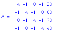
1.1/34 The solution is
| > |
| > |
| > |
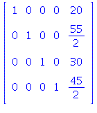
The values of ![]() are the entries in the last column.
are the entries in the last column.
Section 1.2:
1.2/4.
| > |
![table( [( 1, 1 ) = 1, ( 2, 2 ) = 5, ( 3, 3 ) = 9, ( 1, 2 ) = 3, ( 3, 2 ) = 7, ( 3, 1 ) = 5, ( 2, 3 ) = 7, ( 3, 4 ) = 1, ( 2, 1 ) = 3, ( 1, 3 ) = 5, ( 1, 4 ) = 7, ( 2, 4 ) = 9 ] )](images/PS1Sol_14.gif)
| > |
![table( [( 1, 1 ) = 1, ( 2, 2 ) = 1, ( 3, 3 ) = 0, ( 1, 2 ) = 0, ( 3, 2 ) = 0, ( 3, 1 ) = 0, ( 2, 3 ) = 2, ( 3, 4 ) = 1, ( 2, 1 ) = 0, ( 1, 3 ) = -1, ( 1, 4 ) = 0, ( 2, 4 ) = 0 ] )](images/PS1Sol_16.gif)
The pivot columns are columns 1, 2, and 4.
1.2/10
| > |
![table( [( 1, 1 ) = 1, ( 2, 2 ) = -6, ( 1, 2 ) = -2, ( 2, 3 ) = -2, ( 2, 1 ) = 3, ( 1, 3 ) = -1, ( 1, 4 ) = 3, ( 2, 4 ) = 2 ] )](images/PS1Sol_18.gif)
| > |
![table( [( 1, 1 ) = 1, ( 2, 2 ) = 0, ( 1, 2 ) = -2, ( 2, 3 ) = 1, ( 2, 1 ) = 0, ( 1, 3 ) = 0, ( 1, 4 ) = -4, ( 2, 4 ) = -7 ] )](images/PS1Sol_20.gif)
The general solution is
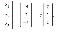 where s is any real number.
1.2/12
| > |

| > |

The general solution is
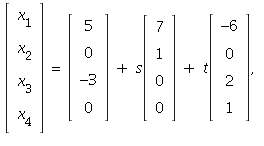 where s, t are any real numbers.
1.2/16 a. System is consistent and solution is unique.
b. System is consistent, but solution is not unique (![]() is a free variable).
is a free variable).
1.2/18 Replace row 2 by row 2, plus (-5) times row 1. The result is
 This augmented matrix represents an inconsistent
system if h = -15. It is consistent for all other values of h, since
in all other cases, we could divide through on the second row
by h + 15 and solve for ![]() .
.
1.2/20. In matrix form, the system is
 Replace row 2 by row 2 plus (-3) times row 1:

a) The system has no solution (is inconsistent) if ![]()
b) The system has a unique solution if ![]() can be anything).
can be anything).
c) The system has infinitely many solutions if ![]() and
and
![]()
1.2/23. Yes. The coefficient matrix is the part of the augmented
matrix corresponding to the left-hand sides of the equations.
If there are three pivot columns, we can solve for three of
the variables in terms of the other two (free) variables.
1.2/24. No. If the last column in the augmented matrix is
a pivot column, then (in the rref) the row containing that
pivot entry must look like: 0 0 0 0 1. This gives an equation
0 = 1, so the system is inconsistent.
1.2/28. It must be true that every column except the last is
a pivot column (no free variables to get solution unique,
and no pivot in the last column, so system is consistent).
1.2/29. If such a system is consistent, then there can
be at most as many basic variables as equations in the
original system. This means there must be at least one
free variable. So there are infinitely many solutions.
1.2/30. The system with augmented matrix
 is such an example. The rref
is
 so the system is inconsistent.
1.2/31. Yes an overdetermined system can be consistent.
The system with augmented matrix
 is an example. The rref is
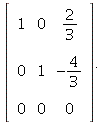
(Note: the third row of the original matrix is the sum of the first
two rows, so it cancels out completely with the row operations.)
Section 1.3
1.3/12.
| > |
![table( [( 1, 1 ) = 1, ( 2, 2 ) = 5, ( 3, 3 ) = 8, ( 1, 2 ) = 0, ( 3, 2 ) = 5, ( 3, 1 ) = 2, ( 2, 3 ) = 0, ( 3, 4 ) = -7, ( 2, 1 ) = -2, ( 1, 3 ) = 2, ( 1, 4 ) = -5, ( 2, 4 ) = 11 ] )](images/PS1Sol_41.gif)
| > |
![table( [( 1, 1 ) = 1, ( 2, 2 ) = 1, ( 3, 3 ) = 0, ( 1, 2 ) = 0, ( 3, 2 ) = 0, ( 3, 1 ) = 0, ( 2, 3 ) = 4/5, ( 3, 4 ) = 1, ( 2, 1 ) = 0, ( 1, 3 ) = 2, ( 1, 4 ) = 0, ( 2, 4 ) = 0 ] )](images/PS1Sol_43.gif)
There is a pivot in the last column, so this system has no solutions.
The vector b is not in the linear combination of the a's.
1.3/14. Same idea as 12:
| > |
![table( [( 1, 1 ) = 1, ( 2, 2 ) = 3, ( 3, 3 ) = 5, ( 1, 2 ) = -2, ( 3, 2 ) = -2, ( 3, 1 ) = 1, ( 2, 3 ) = 7, ( 3, 4 ) = 9, ( 2, 1 ) = 0, ( 1, 3 ) = -6, ( 1, 4 ) = 11, ( 2, 4 ) = -5 ] )](images/PS1Sol_45.gif)
| > |
![table( [( 1, 1 ) = 1, ( 2, 2 ) = 1, ( 3, 3 ) = 1, ( 1, 2 ) = 0, ( 3, 2 ) = 0, ( 3, 1 ) = 0, ( 2, 3 ) = 0, ( 3, 4 ) = -2/11, ( 2, 1 ) = 0, ( 1, 3 ) = 0, ( 1, 4 ) = 245/33, ( 2, 4 ) = -41/33 ] )](images/PS1Sol_47.gif)
This system has a unique solution, giving the scalars
in a linear combination of the columns of A that equals
the vector b.
1.3/16 and 20. You can take any scalars and compute
![]()
The vectors do not lie along the same line,
so the Span is a plane in ![]()
1.3/18.
By looking at the 2nd and 3rd components of a
linear combination ![]()
you can see ![]()
so ![]() Then, from the first components,
Then, from the first components,
![]() (You can also do this
(You can also do this
by reducing to echelon form and seeing when the
system is consistent, of course.)
1.3/22. We just need to force the b to not be
a linear combination of the columns in A. One
easy way to do this is to give A a whole row of
zeroes (say in row 3), but put a nonzero entry in
the third row of b:

(Note the problem just says "A has nonzero entries,"
which is true here, not "A has only nonzero entries."
If you insist that A have only nonzero entries, then
you can get an example, for instance, by making
all the columns of A the same, but b not a scalar
multiple of that vector:
](images/PS1Sol_55.gif)
1.3/25
a. No. This notation ![]() means the set consisting
means the set consisting
of the three columns of A (just those three vectors). b
is not one of those columns.
b. Yes:
| > |
![table( [( 1, 1 ) = 1, ( 2, 2 ) = 3, ( 3, 3 ) = 3, ( 1, 2 ) = 0, ( 3, 2 ) = 6, ( 3, 1 ) = -2, ( 2, 3 ) = -2, ( 3, 4 ) = -4, ( 2, 1 ) = 0, ( 1, 3 ) = -4, ( 1, 4 ) = 4, ( 2, 4 ) = 1 ] )](images/PS1Sol_58.gif)
| > |
![table( [( 1, 1 ) = 1, ( 2, 2 ) = 1, ( 3, 3 ) = 1, ( 1, 2 ) = 0, ( 3, 2 ) = 0, ( 3, 1 ) = 0, ( 2, 3 ) = 0, ( 3, 4 ) = -2, ( 2, 1 ) = 0, ( 1, 3 ) = 0, ( 1, 4 ) = -4, ( 2, 4 ) = -1 ] )](images/PS1Sol_60.gif)
There is a solution of this system (unique in fact). So
b is in W. There are infinitely many vectors in W because
we can use any real scalars in the linear combinations.
c. If ![]() then
then ![]()
This shows ![]() is in W.
is in W.