MATH 134 -- Intensive Calculus for Science 2

Normal probability densities

March 25, 2002

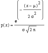
The normal pdf with mean and standard deviation is defined by

> normaldist:=(mu,sigma,x)->exp(-(x-mu)^2/(2*sigma^2))/(sigma*sqrt(2*Pi)):

The value of gives the "center" of the distribution, and the value of describes

how "spread out" it is around the center. Here are some examples. First,

> plot(normaldist(0,1,x),x=-4..4,axes=boxed);

Next, to illustrate what changes as increases -- the bigger

is, the more spread-out the density is (and the lower the peak at is):

> plot({normaldist(1,.2,x),normaldist(1,1,x),normaldist(1,2,x)},x=-3..4,axes=boxed);

On the other hand, fixing , but increasing just shifts the graph to the right:

> plot({normaldist(1,1,x),normaldist(2,1,x),normaldist(3,1,x)},x=-3..7,axes=boxed);

For every normal density function, the probability Prob( <= x <= ) is the same:

> Digits:=20;

> evalf(Int(normaldist(0,1,x),x=0..1));

> evalf(Int(normaldist(12,.03,x),x=12..12.03));

(up to the error from Maple's numerical integration routines!) This says: The probability

that a normally distributed random variable is between its mean and its mean plus its

standard deviation is just a bit more than .34 (or 34%).