MATH 134 -- Intensive Calculus for Science 2

March 21, 2001

Taylor Polynomial Demo

Taylor polynomials for at

> p2:=convert(taylor(cos(x),x=0,3),polynom);

> p4:=convert(taylor(cos(x),x=0,5),polynom);

> p6:=convert(taylor(cos(x),x=0,7),polynom);

> plot({cos(x),p2,p4,p6},x=-Pi..Pi);

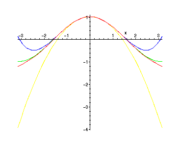
Here the green graph is , the yellow graph is , the blue graph

is , and the red graph is . Intuitively, it is clear that the approximation

of by is getting better as increases. We can make this more precise in

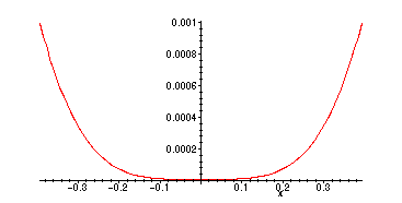
the following way. The function gives the absolute value of the

error in the approximation of by . For all <= x <= the error for

is less than .001 =

> plot(abs(cos(x)-p2),x=-Pi/8..Pi/8);

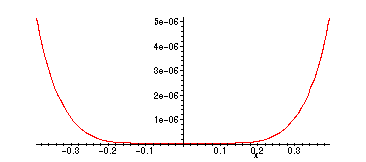
The error for on the same interval is much smaller -- at most

> plot(abs(cos(x)-p4),x=-Pi/8..Pi/8);

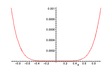
Moreover, the interval where the error with is at most is larger:

> plot(abs(cos(x)-p4),x=-0.95..0.95);

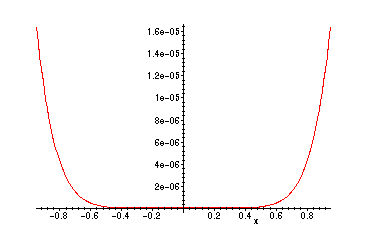
Similarly with , the error on this interval is smaller:

> plot(abs(cos(x)-p6),x=-0.95..0.95);

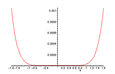
and the interval on which the error with is at most gets larger:

> plot(abs(cos(x)-p6),x=-1.6..1.6);

>