MATH 134 -- Intensive Calculus for Science 2

Slope Fields and Euler's Method in Maple

April 9, 2001

To plot slope fields and approximate solutions of first order

differential equations, we need to begin by loading the DEtools package:

> with(DEtools):

> eqn:=diff(y(x),x) = y(x)*(5-y(x))/4;

To plot a slope field (without any approximate solutions), we can use the DEplot

command as follows: DEplot( eqn, var, x-range, y-range, arrows=SLIM);

where

eqn is the differential equation, entered as above

x-range is the range of x -values to plot

y-range is the range of y -values to plot

arrows=SLIM is an option that controls the way the slope field is plotted

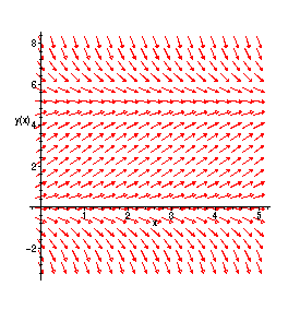
> DEplot(eqn,y(x),x=0..5,y=-3..8,arrows=SLIM);

If we want to see approximate solutions plotted too, we put in initial conditions instead of

the range of y-values, in square brackets, separated by commas, in the form :

DEplot( eqn, var, x-range, initialconds, linecolor=BLACK,arrows=SLIM);

(It is also good to include another option to specify the color these solution graphs will

be drawn with -- the default is a gold-ish color that does not show up well when these

plots are printed!!)

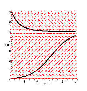
> DEplot(eqn,y(x),x=0..5,[[y(0)=.1],[y(0)=7]],linecolor=BLACK,arrows=SLIM);

Euler's Method is one way to approximate solutions of a differential equation

. Starting from a given ( ), and with a given step size

, we compute further points on an approximate solution graph by the

formulas:

repeated as often as desired (often, you keep going until reaches some desired

stopping value). In Maple, this computation can be done as follows. Say we want

to approximate solutions of with the initial condition

> f:=(x,y) -> 3*x^2-y;

> EulerX[0]:=0; EulerY[0]:=1; DeltaX:=.25;

> for i to 4 do EulerX[i]:=EulerX[i-1] + DeltaX; EulerY[i]:=EulerY[i-1]+f(EulerX[i-1],EulerY[i-1])*DeltaX; od;

> pts:=[[EulerX[0],EulerY[0]],[EulerX[1],EulerY[1]],[EulerX[2],EulerY[2]],[EulerX[3],EulerY[3]],[EulerX[4],EulerY[4]]]:

> ptsplot1:=plot(pts,color=BLUE):

> ptsplot2:=plot(pts,style=point,color=BLACK,symbol=BOX):

> deplot:=DEplot(diff(y(x),x)=3*x^2-y(x),y(x),x=0..1,y=0..1.5,[[y(0)=1]],linecolor=BLACK,arrows=SLIM):

> with(plots):

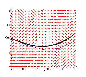
This plot shows:

1) Maple's approximate solution graph (the heavy line)

2) The Euler approximation generated above (the boxes),

which are connected by lighter lines

> display({ptsplot1,ptsplot2,deplot});

In fact, Maple's DEplot command uses a more sophisticated numerical method

and generates a list of approximate points on the solution graph and "connects the

dots" as here to draw the graph!