MATH 392 -- Geometry Through History 

Geodesics on a surface of revolution 

April 20, 2016 

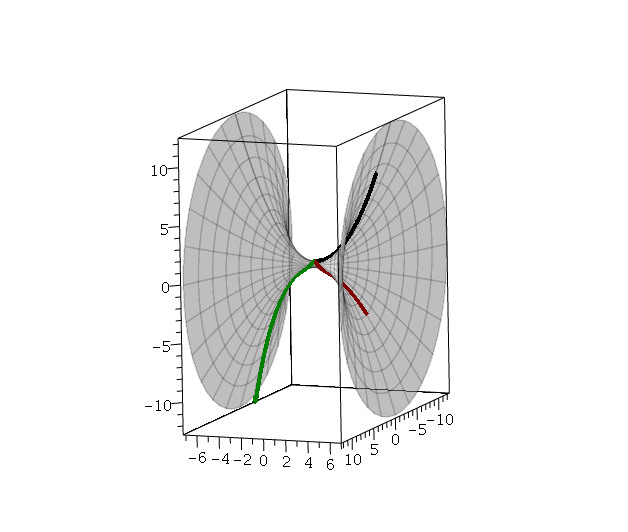
Here are some plots showing geodesics on the surface of revolution given by the following parametrization: 

Note that the meridian curves are parabolas on this surface, but they are not parametrized by arc-length 

as in the general derivation we did in class.   Here is the set-up for the geodesic equations.  We begin by  

plotting the surface, then computing the Christoffel symbols    

(1)

 

(2)

 

 

 

	(3)

 

 

	(4)

 

(5)

 

(6)

 

(7)

 

(8)

 

(9)

 

(10)

 

(11)

 

(12)

 

(13)

 

(14)

 

(15)

 

(16)

 

(17)

 

These are the differential equations for geodesics, entered in Maple format.  These will not have nice explicit solutions in  

elementary functions, so we will need to solve numerically, giving initial values for and their first derivatives. 

This specifies the starting point of the geodesic and its tangent vector at the initial point.  The output 

of the dsolve command is a procedure that computes approximate values for These  

are then substituted into the surface parametrization to give points on the surface.  The curves are 

plotted as lists of points via the pointplot3d commands below: 

(18)

 

(19)

 

(20)

 

(21)

 

The surface and three different geodesics starting at the point plotted in black, red, and green: