Mathematics 173 -- Applied Mathematics 1

A First Boundary Value Problem

We consider the series solution for the BVP:

,

First we check our computation of the Fourier coefficients for

the initial temperature distribution function:

> restart;

> f := x -> x*(L - x);

> assume(m,integer):

> d := m -> (2/L)*int(f(x)*sin(m*Pi*x/L),x=0..L);

> d(m);

We expect that the series should converge to for x in [0, L ].

Let's check this "experimentally". We will define a function of k and x which gives

the k th partial sum of the Fourier series:

> s := (k,x) -> sum(d(n)*sin(n*Pi*x/L),n=1..k);

To plot these partial sum functions and compare with , we will take

> L := 5;

> plot({f(x),s(1,x)},x=0..L);

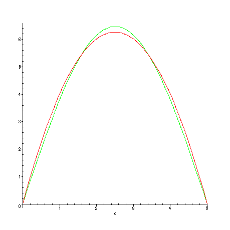
We get close agreement already with -- the largest difference is about 0.4 .

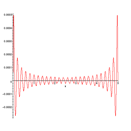
For larger k , the agreement gets even better:

> plot(f(x) - s(50,x),x=0..L);

Next, we will study the corresponding solution of the heat equation obtained as

We take:

> k:=0.1;

Once again, to plot, we will need to compute partial sums of this series. Since

the exponential factors go to zero rapidly as n increases (for t > 0 ), we will

only use a few terms of the series for u (adding in more terms changes the results

very little).

> u := (x,t) -> sum(d(n)*exp(-k*(n*Pi/L)^2*t)*sin(n*Pi*x/L),n=1..3);

> plot3d(u(x,t),x=0..L,t=0..50,axes=BOXED);

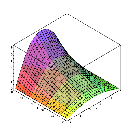
The slices of this plot in the planes t = const. give the temperature functions at each time.

For instance, the slice shows the initial temperature .

Note that as t increases, the temperature at all points of the rod is tending toward zero.

Is this what we expect?

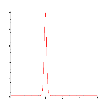
Here is a second example showing an initial temperature distribution showing a

sharp "spike" of heat at one point in the rod. For the previous calculation, we actually

let Maple do all computations of the Fourier coefficients by symbolic methods (getting

exact formulas as we would using integration by parts. For the following initial temperature

function, this would be impractical. Hence we do all the computations to yield numerical

approximations.

> f2:=x->10*exp(-100*(x-2)^2);

> plot(f2(x),x=0..L);

First the Fourier series for f2:

> d2 := n -> evalf((2/L)*Int(f2(x)*sin(n*Pi*x/L),x=0..L));

> s2:=(k,x) -> add(d2(n)*sin(n*Pi*x/L),n=1..k);

Warning, `n` in call to `add` is not local

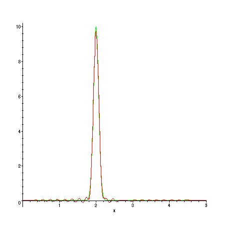
For this function, we need more terms in the Fourier series before we start to

see good agreement with the function!

> plot({f2(x),s2(50,x)},x=0..L);

The corresponding solution of the heat equation:

> u2 := (x,t) -> add(d2(n)*exp(-k*(n*Pi/L)^2*t)*sin(n*Pi*x/L),n=1..50);

Warning, `n` in call to `add` is not local

> plot3d(u2(x,t),x=0..L,t=0..10,axes=BOXED);

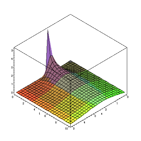
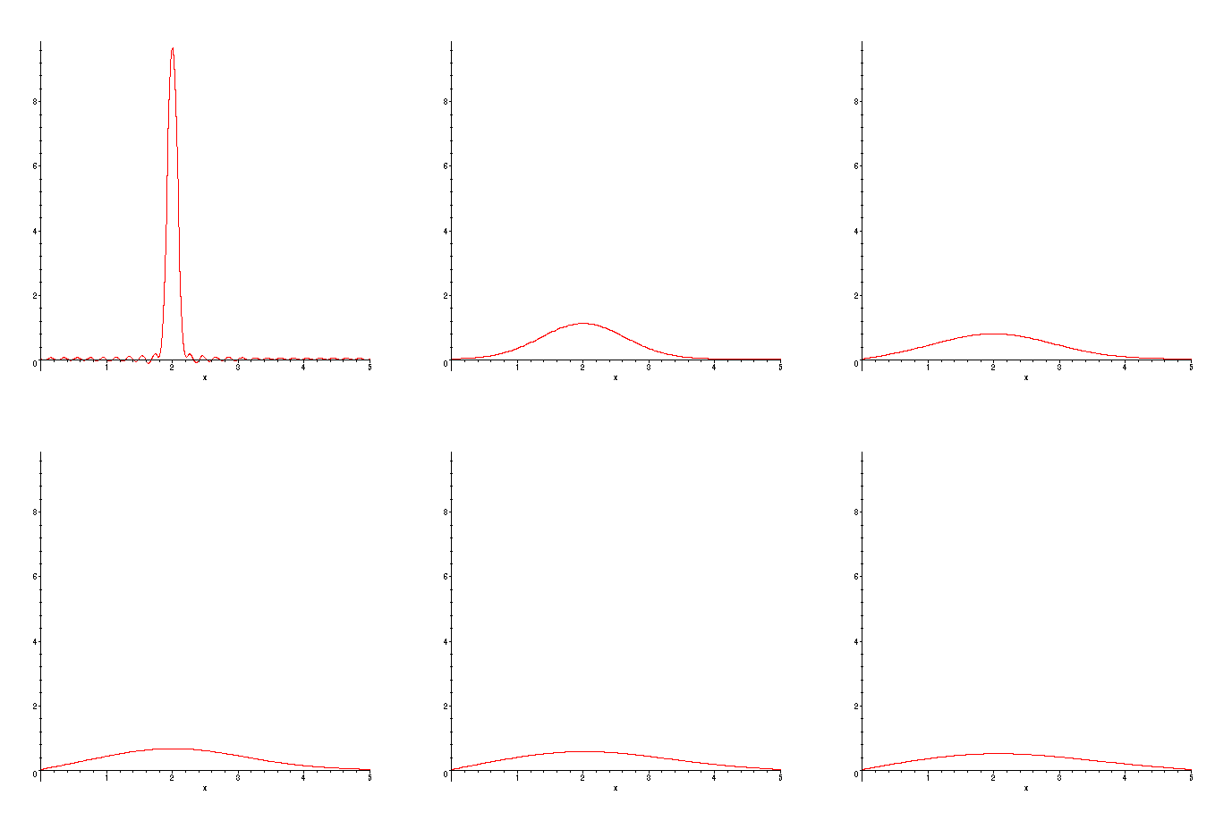
Again, does this look like what we expect? Another way to visualize the passage of time:

> with(plots):

> animate(u2(x,t),x=0..L,t=0..10,frames=50,numpoints=200);

>