Mathematics 174 -- Applied Mathematics 2

Another Convolution Example

Consider the family of Gaussian functions ,

where

> g := (alpha,x) -> exp(-(x/alpha)^2)/(alpha*sqrt(Pi));

> plot({g(2,x),g(1,x),g(1/2,x),g(1/4,x)},x=-4..4,color=red);

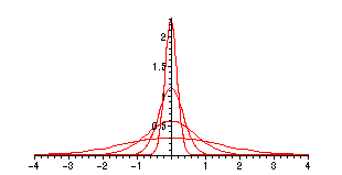
As -> 0+, acquires a taller and taller peak at x = 0, while for all x not

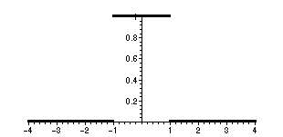
equal to zero. If we convolve with another function like

> f := x -> piecewise(abs(x) < 1, 1, 0);

> plot(f(x),x=-4..4,discont=true,color=black,thickness=3);

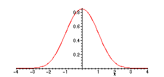
> convo := (alpha,x) -> int(f(t)*g(alpha,x-t),t=-1..1);

N.B. Limits of integration are t = - 1..1 rather than t = , since f(t) is

zero outside the interval t = - 1..1 .

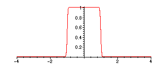
> plot(convo(1,x),x=-4..4);

> plot(convo(.25,x),x=-4..4);

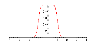
> plot(convo(.05,x),x=-4..4);

>

Note that as +, the graph of the convolution f * tends to approximate f more and

more closely! (This is not really a surprise: What is as ?) However,

for all , the convolution f * is infinitely differentiable (hence continuous).