Mathematics 174 -- Applied Mathematics 2

February 17 - 19, 2000

Bessel Functions and The Vibrating Circular Drumhead

> read "/home/fac/little/public_html/Applied9900/BesselData.m";

Part 1: Eigenfunctions and Eigenvalues for the BVP

> f := BesselJ(m,BesselJZeros(m,n)*r/a);

> simplify(diff(r*diff(f,r),r) - m^2*f/r);

Note: This says that f is an eigenfunction of

with eigenvalue and weight function .

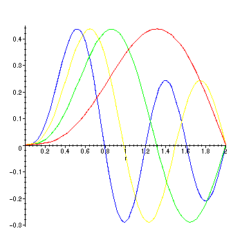
Here are some plots. We fix m = 3, a = 2, and let n vary.

> phi := n -> BesselJ(3,BesselJZeros(3,n)*r/2);

> plot({phi(1),phi(2),phi(3),phi(4)},r = 0..2);

Note that the same patterns of zeros that we know for eigenfunctions of regular Sturm-Liouville problems

are also true here!

Part 2: Fourier - Bessel Series

Given any piecewise smooth function on [0,a], and given any particular

nonnegative integer m, we can expand in a Fourier-Bessel series :

using the eigenfunctions , where are the

positive roots of , and the Fourier-Bessel coefficients are given by

There is a point-wise convergence theorem valid here too, just as for the eigenfunction

expansions for regular Sturm-Liouville problems.

For instance, let's consider with a = 2, and m = 0. (These are chosen

arbitrarily -- as we will see in later examples, the value of m that must be used is

often determined by other conditions in actual problems.)

> with(plots):

> psi := r -> 1 - r^2;

> phi := n -> BesselJ(0,BesselJZeros(0,n)*r/2);

The Fourier-Bessel coefficients are given by the formula above, with m = 0:

> a := n -> evalf(Int(psi(r)*phi(n)*r,r = 0 .. 2))/evalf(Int(phi(n)^2*r,r = 0 .. 2));

As always, to plot, we need to look at partial sums of the Fourier-Bessel series:

> PS := N -> add(a(n)*phi(n),n=1..N);

Warning, `n` in call to `add` is not local

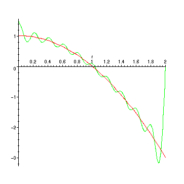
> FBPlot:=plot({psi(r),PS(20)},r=0..2):

> display(FBPlot);

Note: Because all the eigenfunctions have the value zero at r = 2, there will be jump

(Gibbs phenomenon-like) effects there. A similar phenomenon is happening at r = 0.

For each fixed r in (0,2), since this is continuous on the open interval,

the Fourier-Bessel series will converge to . However, the over- and under-shoots

at the endpoints for the partial sums will persist (but get closer to the ends and "thinner")

no matter how large N is.

Part 3: The Vibrating Circular Drumhead

For the boundary value problem:

we use Fourier-Bessel expansions as above to find the solution. Since the initial data

is independent of , only the terms with m = 0 in our general expansions are

needed:

> beta := piecewise(r < .25,-1,0):

> phi := n -> BesselJ(0,BesselJZeros(0,n)*r/2);

The Fourier-Bessel coefficients are given by the formula above

> A := n -> (2/BesselJZeros(0,n)*1)*evalf(Int(beta(r)*phi(n)*r,r = 0 .. 2))/evalf(Int(phi(n)^2*r,r = 0 .. 2));

As always, to plot, we need to look at partial sums of the Fourier-Bessel series:

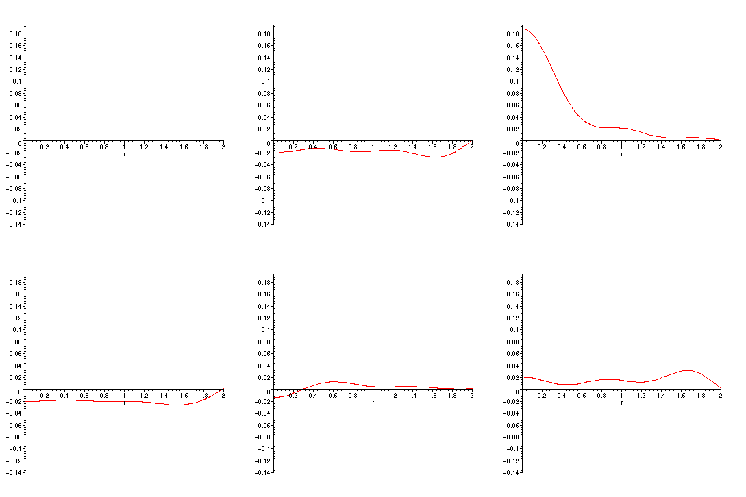
> PSu := add(A(n)*phi(n)*sin(BesselJZeros(0,n)*1*t/2),n=1..5):

> animate(PSu,r=0..2,t=0..10,frames=50);

> save FBPlot,PSu,"/home/fac/little/public_html/Applied9900/BesselData.m";

>