Mathematics 174 -- Applied Mathematics 2

The Averaging Filter

= ( f * B)( x ), where B( x ) = 1 on [0,1] and zero elsewhere.

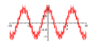
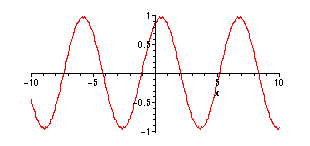
For example, here are the graphs of an input signal and the output under the

averaging filter. Think of the input signal as , plus some higher

frequency "noise":

> f:=x->cos(x)+15*cos(20*x)/100-cos(30*x)/5;

> plot(f(x),x=-10..10,numpoints=300);

> Gamma := (input,x) -> evalf(Int(input(s),s=x-1..x));

> plot(Gamma(f,x),x=-10..10,numpoints=300);

Note that the averaging seems to have largely "smoothed out" the noise and given something like

a horizontally shifted (and vertically scaled) version of the input. In fact, the magnitude

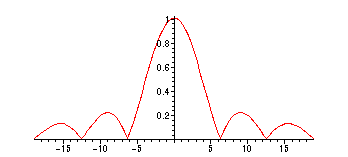
response function of the filter is given by

> plot(sqrt((2-2*cos(omega))/omega^2),omega=-6*Pi..6*Pi);

We do not have a sharp cut-off frequency here between the pass-band and the stop-band,

but this is also an example of a low-pass filter. And this one is causal, unlike the brick-wall

ideal low-pass filter. For examples like this one, the pass-band is taken (by definition or

convention) to be the interval of -values where the magnitude response is greater than

or equal to = .707 (approx). Here, that happens for in [ , ]:

> fsolve(sqrt((2-2*cos(omega))/omega^2)-1/sqrt(2),omega);

The value of the magnitude response at

> evalf(subs(omega=1,sqrt((2-2*cos(omega))/omega^2)));

gives the vertical scaling factor between the amplitude of the input and the amplitude of the

output.

>