Mathematics 174 -- Applied Mathematics 2

Lab 5 (FFT) Solutions

> restart;

> readlib(FFT):

B) Example 2

> f := x->25*cos(194*x):

> inpR:=array([seq( evalf(f(j*2*Pi/1024)),j=0..1023)]):

> inpI:=array([seq(0,j=0..1024)]):

> FFT(10,inpR,inpI):

> FPSpoints:=[seq([k,sqrt(inpR[k]^2+inpI[k]^2)],k=1..1024)]:

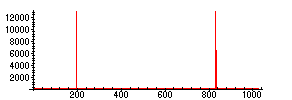
> plot(FPSpoints);

Recall that in Maple, the DFT sequence term gives an approximation to , where

is the "analog" Fourier transform of f. If , then this analog FT can be

obtained like this. The FT of the window function is similar to that in the worked example,

but the height of the central peak is proportional to the width of the window :

> FW:=int(exp(I*omega*x),x=0..Omega)/(2*Pi):

> assume(omega,real);

> FPS:=abs(subs(Omega=2*Pi,FW)):

> plot(FPS,omega=-20..20,numpoints=300);

The height of the central peak is . By the linearity and modulation properties of the

Fourier Transform, the FT of looks like two shifted copies of this,

scaled by 1/2 and superposed (i.e. added) -- centers shifted left and right to - and + B.

Going now to the DFT , recall once again that the DFT sequence term gives an approximation

to , where is the analog FT of . The periodicity of the 1024-point

DFT implies that the DFT of A cos( Bx ) will have peaks at approximately and

. The height of the peak should be . For the example above

with , this gives:

> 512*25;

which agrees closely with the plot.

D) Using the "mystery signal itself"

> read "/home/fac/little/public_html/Applied9900/mystery.m";

> FFT(10,MystR,MystI):

> FPSpoints:=[seq([k,sqrt(MystR[k]^2+MystI[k]^2)],k=1..1024)]:

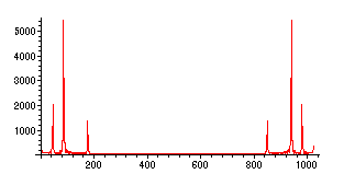
> plot(FPSpoints);

Band-pass filter with pass-band: 60 <= | | <= 120 (MystR and MystI are now the FT of the

mystery signal.) So in the frequency domain, we want:

> H:=[seq(0,j=1..59),seq(1,j=60..120),seq(0,j=121..903),seq(1,j=904..964),seq(0,j=965..1024)]:

The following is OK for the product since the imaginary part of H is zero.

> FiltR:=array([seq(MystR[k]*H[k],k=1..1024)]):

> FiltI:=array([seq(MystI[k]*H[k],k=1..1024)]):

> iFFT(10,FiltR,FiltI);

> plot([seq([2*Pi*(j-1)/1024,FiltR[j]],j=100..200)]);

The imaginary part is about 2 orders of magnitude smaller, so we will ignore it.

E) FFT for convolution

> f:=x->exp(-2*(x-3)^2):

> g:=x->exp(-3*(x-2)^2):

> plot({f,g},0..10);

Sampling f and g:

> Ref:=array([seq(evalf(f(10*i/1024)),i=0..1023)]):

> Imf:=array([seq(0,i=0..1023)]):

> Reg:=array([seq(evalf(g(10*i/1024)),i=0..1023)]):

> Img:=array([seq(0,i=0..1023)]):

> FFT(10,Ref,Imf):

> FFT(10,Reg,Img):

Real and imaginary parts of these DFTs are non-zero. Hence to multiply, we must do

the following. (Also, Maple's FFT does not include our factor , so the DFT of the

convolution is just the product of the FFTs, without the extra factor of ):

> ReProd:=array([seq(Ref[k]*Reg[k]-Imf[k]*Img[k],k=1..1024)]):

> ImProd:=array([seq(Ref[k]*Img[k]+Imf[k]*Reg[k],k=1..1024)]):

> iFFT(10,ReProd,ImProd):

We want to plot the result on the interval . So the first coordinates

of the points we plot are . Recall yet again that the DFT sequence term using

samples of any function f gives an approximation to , where is the

analog FT of . The product of the DFT's gives the times the DFT of the

convolution -- i.e. our result is times what we want!! We need to multiply

by = 10/1024 to get the correct vertical scaling:

> Points:=[seq([10*(i-1)/1024,ReProd[i]*10/1024],i=1..1024)]:

> plot(Points);

Again, the imaginary parts are very small , so we ignore them. By problem II on Problem Set 5

we know a formula for the convolution of and

namely: * = where . Our first gaussian is

(that is, and c = 2). Similarly, g( x ) = (that is, and ).

By our formula f * g = where = and c + d = 5 (which agrees with

the center of the peak in the plot above!)

> plot({Points,(Pi/sqrt(6))*1/sqrt(2*Pi*5/12)*exp(-(x - 5)^2/(2*(5/12)))},x=0..10);

Note: These are so close that it's hard to see that there are two plots here!

>