MATH 136 -- Advanced Placement Calculus 

Taylor Polynomials Examples 

December 7, 2009 


We have seen the description of the Taylor (or MacLaurin) 

polynomials of a given function.  For example, the 4th degree 

polynomial for  cos(x)is the polynomial given below: 


`assign`(p4, convert(taylor(cos(x), x = 0, 5), polynom)); 1 

`+`(1, `-`(`*`(`/`(1, 2), `*`(`^`(x, 2)))), `*`(`/`(1, 24), `*`(`^`(x, 4)))) (1)
 

This polynomial can be used to approximate cos(x)for  xclose to zero: 

`assign`(approx, `+`(1, `-`(`/`(`*`(`^`(.3, 2)), `*`(factorial(2)))), `/`(`*`(`^`(.3, 4)), `*`(factorial(4))))); 1 

.9553375000 (2)
 

`assign`(exact, cos(.3)); 1 

.9553364891 (3)
 

`assign`(p4error, `+`(exact, `-`(approx))); 1 

-0.10109e-5 (4)
 

`assign`(approx, subs(x = .9, p4)); 1 

.6223375000 (5)
 

`assign`(exact, cos(.9)); 1 

.6216099683 (6)
 

`assign`(p4error, `+`(exact, `-`(approx))); 1 

-0.7275317e-3 (7)
 

`assign`(approx, subs(x = 1.5, p4)); 1 

0.859375000e-1 (8)
 

`assign`(exact, cos(1.5)); 1 

0.7073720167e-1 (9)
 

`assign`(p4error, `+`(exact, `-`(approx))); 1 

-0.1520029833e-1 (10)
 

In fact, here is the graph of  p4x  and  cos(x)for  `and`(`<=`(-3, x), `<=`(x, 3)); -1plot([p4, cos(x)], x = -3 .. 3, color = [black, red], scaling = constrained); 1 

Plot_2d
 

(The Taylor polynomial is in black; the cosine graph is in red.  Note how close the graphs 

are for  or so.   


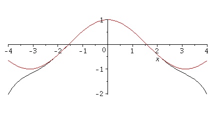
If we increase the degree of the polynomial, the agreement is even closer close to zero, and  

it stays closer over longer intervals: 


Taylor polynomial of degree 6 and cos(x); -1 


plot([convert(taylor(cos(x), x = 0, 7), polynom), cos(x)], x = -4 .. 4, color = [black, red], scaling = constrained); 1
 

Plot_2d
 

Taylor polynomial of degree 8 and cos(x); -1 


plot([convert(taylor(cos(x), x = 0, 9), polynom), cos(x)], x = -4 .. 4, color = [black, red], scaling = constrained); 1
 

Plot_2d
 

Taylor polynomial of degree 20 and cos(x); -1 


plot([convert(taylor(cos(x), x = 0, 21), polynom), cos(x)], x = -10 .. 10, y = -5 .. 5, color = [black, red], scaling = constrained); 1
 

Plot_2d