MONT 106N -- Identifying Patterns 

October 2, 2009

A "fat-tail" distribution 

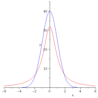
One very simple (i.e. defined by a mathematically simple formula) example of a  

"fat-tail" distribution is shown here in red, together with the normal curve 

in blue for comparison.  The horizontal axis is measured in standard units 

for the normal curve and the vertical axis is in %/standard unit, as usual.  

>

 

>

 

By way of comparison:  The area under the normal curve (blue) 

between 2 and is about 2.5%.  The area under the "fat-tail" 

curve between 2 and is about 9.5% 

>