MATH 373 -- Applied Mathematics (PDE)

February 20, 2001 -- First examples of Fourier Series

A) Consider the function f(x) = - 1 if <= x < 0, and 1 if 0 <= x <=

The Fourier coefficients are given by

> assume(n,integer);

> f := x->piecewise(x<0,-1,1):

> af := n->int(f(x)*cos(n*x),x=-Pi..Pi)/Pi;

Since f is an odd function, for all n >= 0:

> af(n);

> bf := n->int(f(x)*sin(n*x),x=-Pi..Pi)/Pi;

> bf(n);

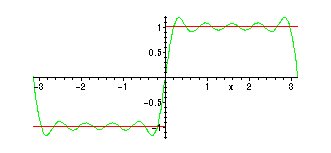
To visualize the Fourier series, we can plot partial sums:

> PSf:=(N,x)->add(bf(n)*sin(n*x),n=1..N);

Warning, `n` in call to `add` is not local

> plot({f(x),PSf(10,x)},x=-Pi..Pi);

B) Now, consider g(x) = on

> g:=x -> x^2;

> ag := n->int(g(x)*cos(n*x),x=-Pi..Pi)/Pi;

> ag(0);

> ag(n);

> bg := n->int(g(x)*sin(n*x),x=-Pi..Pi)/Pi;

Now, the coefficients are zero, because g is even.

> bg(n);

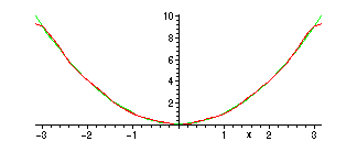
To visualize the Fourier series, we can plot partial sums:

> PSg:=(N,x)->ag(0)/2+add(ag(n)*cos(n*x),n=1..N);

Warning, `n` in call to `add` is not local

> plot({g(x),PSg(5,x)},x=-Pi..Pi);

Note that the approximation to the function g given by the partial sum of the

Fourier series seems much closer in this case than in example A.