Mathematics 373 -- Applied Mathematics 1 (PDE)

February 27, 2001

Fourier Sine and Cosine Series, Solutions of the Heat Equation

Consider the function on the interval [0,3]

(This could represent something like an initial temperature distribution in a heat

conduction problem.)

> f := x -> piecewise(x < 3/2, x, x >= 3/2, exp(-x));

In our work on BVP for the heat equation, we would expand functions like this in series

using the appropriate eigenfunctions for the problem at hand. Two particular cases

were the Fourier sine series:

where

and the Fourier cosine series

where

Both of these are examples of general Fourier series.

The Fourier Sine series of f converges to the odd extension of f on [-3,3]

at points of continuity, and to the average of the one-sided limits at jumps:

>

> B := n -> 2*evalf(Int(f(x)*sin(n*Pi*x/3),x=0..3))/3;

> ss := (k,x) -> add(B(n)*sin(n*Pi*x/3),n=1..k);

Warning, `n` in call to `add` is not local

> with(plots):

> FP:=plot(f(x),x=0..3,color=blue,discont=true):

> SP:=plot(ss(20,x),x=-3..3,color=red):

> display({FP,SP});

On the other hand, the Fourier cosine series for f converges to the even extension of f on [-3,3]

at points of continuity, and to the average of the one-sided limits at jumps:

> A0 := evalf(Int(f(x),x=0..3))/3;

> A := n -> 2*evalf(Int(f(x)*cos(n*Pi*x/3),x=0..3))/3;

> sc := (k, x) -> A0 + add(A(n)*cos(n*Pi*x/3),n=1..k);

Warning, `n` in call to `add` is not local

> CP := plot(sc(20,x),x=-3..3):

> display({FP,CP});

On larger intervals, the sine and cosine series converge to the periodic extensions of the odd and even

extensions, respectively.

Now, we consider using these sine and cosine series to develop the series solutions

for boundary value problems. First we will study:

, (ends of the wire held at zero temperature)

First we check our computation of the Fourier coefficients for

the initial temperature distribution function:

> restart;

> f := x -> x*(L - x);

> assume(m,integer):

Since the eigenfunctions of the problem are the , we use a Fourier

sine series to represent the initial temperature distribution:

> b := m -> (2/L)*int(f(x)*sin(m*Pi*x/L),x=0..L):

> b(m);

By Dirichlet's theorem, since f( x ) is continuous, we know

that the series will converge to for all x in [0, L ].

Let's check this "experimentally". We will define a function of k and x which gives

the k th partial sum of the Fourier sine series:

> S := (N,x) -> add(b(n)*sin(n*Pi*x/L),n=1..N);

Warning, `n` in call to `add` is not local

To plot these partial sum functions and compare with , we will take

> L := 5;

> plot({f(x),S(5,x)},x=0..L);

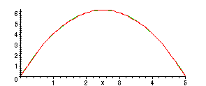
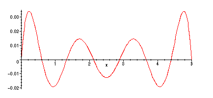
We get very close agreement already with -- the largest difference is about 0.04:

> plot(f(x) - S(5,x),x=0..L);

Next, we will study the corresponding solution of the heat equation obtained as

We take:

> k:=0.1;

Once again, to plot, we will need to compute partial sums of this series. Since

the exponential factors go to zero rapidly as n increases (for t > 0 ), we will

only use a few terms of the series for u (adding in more terms changes the results

very little).

> u := (x,t) -> add(b(n)*exp(-k*(n*Pi/L)^2*t)*sin(n*Pi*x/L),n=1..3);

Warning, `n` in call to `add` is not local

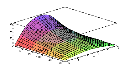
> plot3d(u(x,t),x=0..L,t=0..50,axes=BOXED);

>

The slices of this plot in the planes t = const. give the temperature functions at each time.

For instance, the slice shows the initial temperature .

Note that as t increases, the temperature at all points of the rod is tending toward zero.

Is this what we expect?

Next, we cosider the BVP:

, (ends of the wire insulated )

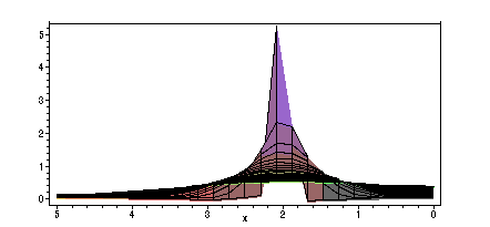
Here the initial temperature shows a sharp "spike of heat" concentrated

around x = 2

> f2:=x->10*exp(-100*(x-2)^2);

> plot(f2(x),x=0..L);

The eigenfunctions for the equation in the space variable x are . So, we use

a Fourier cosine series for this example. (N.B. we are integrating numerically here, not symbolically)

> a2 := n -> evalf((2/L)*Int(f2(x)*cos(n*Pi*x/L),x=0..L));

> S2:=(N,x) -> a2(0)/2 + add(a2(n)*cos(n*Pi*x/L),n=1..N);

Warning, `n` in call to `add` is not local

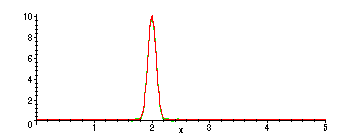
For this function, we need more terms in the Fourier series before we start to

see good agreement with the function!

> plot({f2(x),S2(50,x)},x=0..L);

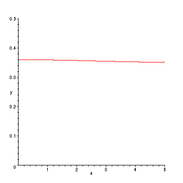
The corresponding solution of the heat equation:

> u2 := (x,t) -> a2(0)/2+add(a2(n)*exp(-k*(n*Pi/L)^2*t)*cos(n*Pi*x/L),n=1..50);

Warning, `n` in call to `add` is not local

> plot3d(u2(x,t),x=0..L,t=0..10,axes=BOXED);

> plot(u2(x,100),x=0..L,y=0..(0.5));

>