MATH 373 -- Applied Mathematics (PDE)

Final Problem Set -- Selected Solutions

I A)

The initial string shape:

> f:=piecewise(x<2,0,x<3,5*(x-2)*(3-x),x<5,0);

The eigenfunctions of the boundary value problem

X'' = - X

X(0) = X(5) = 0

are X( x ) = , n >= 1. The corresponding solution of

the 1D wave equation looks like:

Since , it follows that for all n . The come from the usual

coefficient formulas for a Fourier sine series for the initial string shape on [0,5]

> A:=n->evalf(2*Int(f*sin(n*Pi*x/5),x=0..5)/5);

The partial sum of the Fourier sine series for the initial string shape

> PSFS:=(N,x)->add(A(n)*sin(n*Pi*x/5),n=1..N);

Warning, `n` in call to `add` is not local

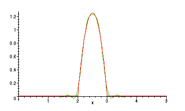
Taking N = 25 gives close agreement with the initial string shape above.

> plot({f,PSFS(25,x)},x=0..5);

> PSu:=(N,x,t)->add(A(n)*sin(n*Pi*x/5)*cos(n*Pi*t/5),n=1..N);

Warning, `n` in call to `add` is not local

> with(plots):

> animate(PSu(20,x,t),x=0..5,t=0..10,frames=30,color=blue);

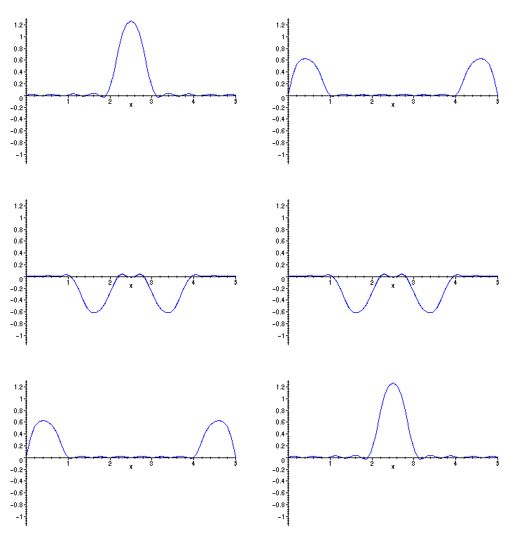
The animation shows the intial peak between x = 2 and x = 3 splitting up into

two peaks of one half the height, one moving left, one moving right. When those

peaks reach the endpoints at x = 0,5 they are reflected so that they move back in

the opposite direction. They are also reflected across the x - axis in the process.

The smaller peaks then "recombine" momentarily below the x - axis, continue

moving in their new directions until they are reflected in the same way at

the opposite endpoints. The cycle then repeats.

D) The reflection of waves at the endpoints seen above can be explained using

the result of part C, which says that the D'Alembert solution of the problem

,

namely , where F is the odd periodic extension of

f , restricted to the interval [0,5] in x, equals the solution of our problem.

The graph of the odd periodic extension, F( x ) has peaks like that in the graph

of f, but below the x-axis, in the intervals [-13, -12], [-3,-2], [ 7,8], [17,18]

etc. In the D'Alembert solution we have two traveling waves, one moving

to the left at constant speed 1, one moving to the right at the same speed. Between

t = 2 and t = 7, for instance, when the plot above shows the reflected wave below

the x-axis, we are seeing the portions of the right-moving and left-moving

waves from the D'Alembert solution that started out in [-3,-2] (moving right),

and [7,8] (moving left) respectively. (In a physical string, the waves really are

reflected by the endpoints, but that behavior "comes mathematically" from the

fact that the restriction of the D'Alembert solution with the odd periodic

initial data is another way to write the solution of this problem.)

III.

A) The three ODE's from this problem are

T ' = -

'' =

R '' + R + ( ) R = 0

The boundary condition , all says R'(a) = 0.

B) The fact that has an infinite sequence where

'( ) = 0 follows from the Mean Value Theorem. Because

we know that the Bessel function has an infinite sequence of zeros,

the numbers we called in class, on each interval between

two consecutive zeros and of there is some

where the derivative is zero. Note: If m <> 1, then

is also a zero of '

C) As we saw in the Bessel function lab, we have the following fact:

> ff:=BesselJ(m,c*r);

> simplify(diff(r*diff(ff,r),r) - (m^2/r)*ff);

This says that if L is the Sturm Liouville operator L(f) = (r f ')' - f , and

= , then L( ) = - . We can then try to choose c a function

satisfying the boundary condition '( a ) = 0. This leads to the condition that

for some n >= 0. The eigenfunctions are

, eigenvalue

and also , eigenvalue 0 if m = 0

D) The initial temperature function in our problem is radially symmetric --

it does not depend on theta. The solutions of the equation for from

part A of this problem are . So the only case

where we get a product solution of the heat equation with u independent

of is if .

We need to derive approximations to the first few zeros of the

derivative of

> plot(BesselJ(0,z),z=0..22);

> mu01:=fsolve(diff(BesselJ(0,z),z)=0,z,z=3..5);

> mu02:=fsolve(diff(BesselJ(0,z),z)=0,z,z=6..8);

> mu03:=fsolve(diff(BesselJ(0,z),z)=0,z,z=9..11);

> mu04:=fsolve(diff(BesselJ(0,z),z)=0,z,z=13..14);

> mu05:=fsolve(diff(BesselJ(0,z),z)=0,z,z=16..17);

> mu06:=fsolve(diff(BesselJ(0,z),z)=0,z,z=19..20);

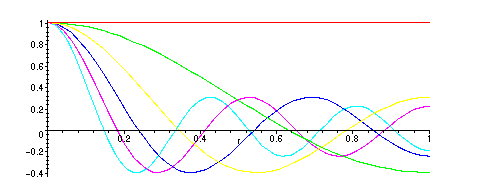
Eigenfunctions are given by 1 (eigenvalue zero) and

BesselJ(0, ), where is one of the zeroes of BesselJ(0,z):

> plot({1,BesselJ(0,mu01*r),BesselJ(0,mu02*r),BesselJ(0,mu03*r),BesselJ(0,mu04*r),BesselJ(0,mu05*r)},r=0..1);

The initial temperature:

> f:=exp(-(r-1/2)^2);

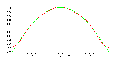
The Fourier-Bessel series for f will look like

, where and

as above. We want to include the term with n = 0 here

too, since m = 0.

> a0:=evalf(Int(f*r,r=0..1))/evalf(Int(r,r=0..1));

> a1:=evalf(Int(f*BesselJ(0,mu01*r)*r,r=0..1))/evalf(Int(BesselJ(0,mu01*r)^2*r,r=0..1));

> a2:=evalf(Int(f*BesselJ(0,mu02*r)*r,r=0..1))/evalf(Int(BesselJ(0,mu02*r)^2*r,r=0..1));

> a3:=evalf(Int(f*BesselJ(0,mu03*r)*r,r=0..1))/evalf(Int(BesselJ(0,mu03*r)^2*r,r=0..1));

> a4:=evalf(Int(f*BesselJ(0,mu04*r)*r,r=0..1))/evalf(Int(BesselJ(0,mu04*r)^2*r,r=0..1));

> a5:=evalf(Int(f*BesselJ(0,mu05*r)*r,r=0..1))/evalf(Int(BesselJ(0,mu05*r)^2*r,r=0..1));

> a6:=evalf(Int(f*BesselJ(0,mu06*r)*r,r=0..1))/evalf(Int(BesselJ(0,mu06*r)^2*r,r=0..1));

> plot({f,a0+a1*BesselJ(0,mu01*r)+a2*BesselJ(0,mu02*r)+a3*BesselJ(0,mu03*r)+a4*BesselJ(0,mu04*r)+a5*BesselJ(0,mu05*r)+a6*BesselJ(0,mu06*r)},r=0..1);

The solution of the heat equation (partial sum approximation):

> u:=a0+a1*BesselJ(0,mu01*r)*exp(-mu01^2*t)+a2*BesselJ(0,mu02*r)*exp(-mu02^2*t)+a3*BesselJ(0,mu03*r)*exp(-mu03^2*t)+a4*BesselJ(0,mu04*r)*exp(-mu04^2*t)+a5*BesselJ(0,mu05*r)*exp(-mu05^2*t)+a6*BesselJ(0,mu06*r)*exp(-mu06^2*t);

> animate3d([r*cos(theta),r*sin(theta),u],r=0..1,theta=0..2*Pi,t=0..3);

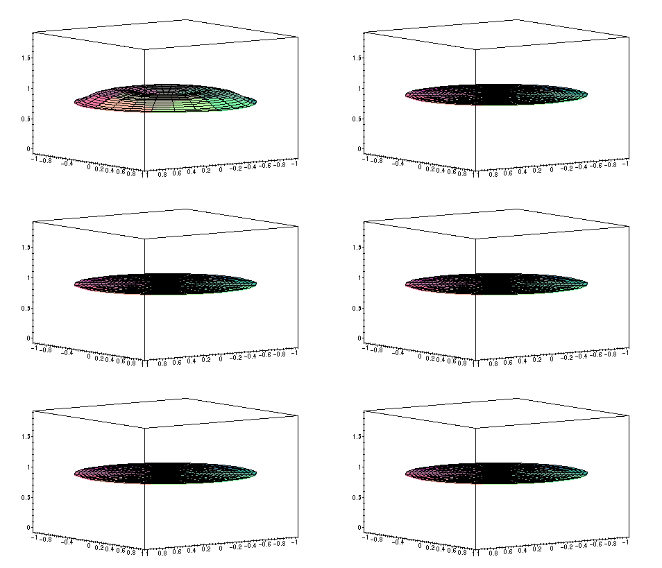
The heat energy in the plate quickly spreads out evenly, tending to an equilibrium solution

where the temperature is constant throughout the plate.