CSCI 363 Computational Vision--Spring 2023
Assignments
Home | | Schedule | | Assignments | | Lecture Notes
Assignment 6, Due Thursday, April 20
This assignment contains two programming problems. In one you will create
a movie to demonstrate the stereo-kinetic-effect, and experiment
with parameters that affect the power of this effect. In the second,
you will compute the optic flow field for a given set of observer motion
parameters. The initial code for the programming problems
are contained in the ~csci363/assignments/assign6 subdirectory
on radius. After copying this folder to your own assign6 directory, set the Current Directory
in MATLAB to this folder.
Problem 1: The Stereokinetic Effect
If an object simply undergoes pure rotation in the image plane, it does not generate 2-D
image motion that can be used to recover its 3-D shape. There are some patterns, however,
that yield a percept of 3-D shape when they are just rotating rigidly in the image. A
particularly striking example of such a pattern is shown below. A movie of this pattern
rotating can be found at a website developed by Michael Bach
(http://www.michaelbach.de/ot/mot-ske/index.html).
This phenomenon is known as the stereokinetic effect. In this problem, your first step
will
be to write a MATLAB function named ske that creates a movie of the pattern shown
below, rotating around its center. This function can be implemented in a way that allows you to
create a variation on this pattern that highlights the basis for perceiving 3-D shape from this
moving image.
There are two functions related to this problem contained in
the assign6 directory that you copied. The function circlePoints generates
x,y coordinates of
a set of points evenly spaced around a circle. The inputs to this function are the
x,y coordinates of the center of the circle, the radius of the circle, and
the number of sample points around its perimeter. This
function returns two vectors containing the x and y coordinates.
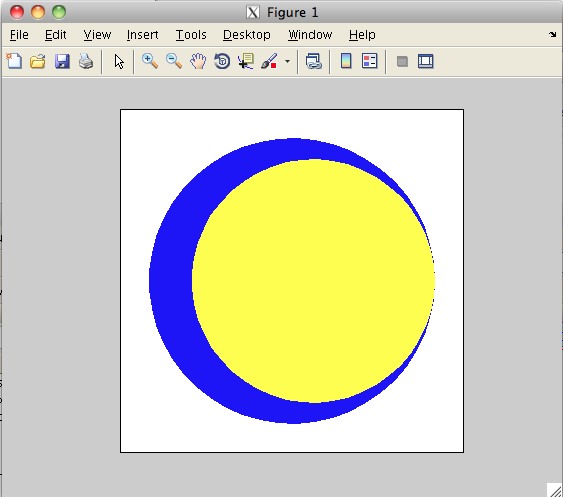
The ske function
creates a movie of a yellow circle rotating inside a larger stationary circle as in the
image below:
The parameter
npts specifies the number of points used to draw the circles. Smaller numbers
of points (e.g. 10) will show polygons, rather than circles. Larger numbers of points (e.g. 50)
will
show smoother circles. The movie is a
sequence of frames stored in
a vector of MATLAB structures. This function uses two built-in functions,
fill
and getframe. The fill function draws a filled-in
polygon, given the x and y coordinates of points around its
perimeter. The getframe function creates a snapshot of the picture displayed in the
current figure window. The built-in movie function can then be
used to display the frames of the movie. The inputs to movie are a vector of
structures
containing the movie frames, the number of times to show the movie, and the rate of presentation
of the frames, specified as the number of frames per second. The ske and
movie functions can be called as shown below:
    >> skeMovie = ske(50);

    >> movie(skeMovie, 2, 10);
Note: If you are logged in remotely, the movie will be very slow and not very smooth, particularly if you are not on campus. To see the full KDE, you should probably try logging in to one of the NUCs in the Swords 219 lab.
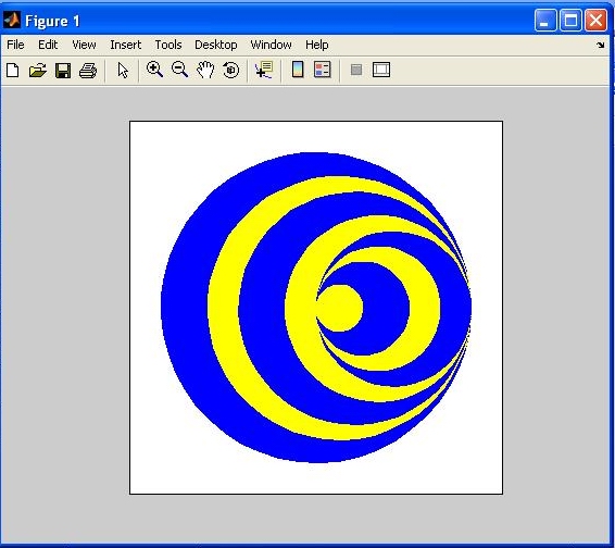
Your assignment is to complete the ske(npts) function so that it shows the complete
ske
rotating figure as diagrammed in the first image above.
Your ske function should return the frames of a movie in which the ske cone pattern
is rotated around its center (for simplicity, the largest blue circle should be centered
at the origin, (0,0)).
Study the ske function to see how it works. Note that to create the movie, first
a circle is created using circlePoints that describes the motion of the center of the
inner yellow circle. In this case it is a circle of radius 15, centered at the origin.
The coordinates of the center of this circle for each frame of the movie
are stored in the vectors: xc1 and yc1, each of which contain 50 values.
For each movie frame created inside the for loop, circlePoints is used
to draw a circle of radius 85 around
the center location, xc1(frame), yc1(frame), for that frame.
To complete the image use the following parameters for the rotating circles:
| Circle number | Radius of motion of center coordinates | Radius of circle | color |
| Circle 1 | 15 | 85 | yellow |
| Circle 2 | 25 | 75 | blue |
| Circle 3 | 40 | 60 | yellow |
| Circle 4 | 50 | 50 | blue |
| Circle 5 | 40 | 40 | yellow |
| Circle 6 | 30 | 30 | blue |
| Circle 7 | 20 | 20 | yellow |
Note that the stationary outer blue circle is not included in the table. The first circle
listed
is the circle already in the ske function you downloaded. You must add the other 6
circles.
Feel free to change the colors in the pattern - it is easiest to use the 8 basic colors that can be specified with a single character (r(red), g(green), b(blue), m(magenta), c(cyan), y(yellow), w(white) and k(black)).
When you are done, turn in a hard-copy of your ske.m file, and upload a copy of the ske.m file to Canvas.
Problem 2: Recovering Observer Motion
Part a: The following equations specify the x and
y components of the image velocity (Vx,Vy)
as a function of the movement of the observer (translation
(Tx,Ty,Tz) and rotation
(Rx,Ry,Rz)) and depth
Z(x,y):
Vx = (-Tx + xTz)/Z + Rxxy -
Ry(x2+1) + Rzy
Vy = (-Ty + yTz)/Z +
Rx(y2 + 1) - Ryxy - Rzx
Write a function setupImageVelocities that computes the image velocity
field that results from a movement of the observer:
function [vx vy xfoe yfoe] = setupImageVelocities(Tx,Ty,Tz,Rx,Ry,Rz,zmap)
The input zmap is a 2-D matrix of the depths of the surfaces that project
to each image location. The output matrices vx and vy should
be the same size as the input zmap. Assume that the origin of the
x,y image coordinate system is represented at the center of the
zmap, vx and vy matrices. The indices of these matrices should
also be scaled to obtain the x and y coordinates that are
used in the above equations. In particular, let i and j
represent the indices of the zmap, vx and vy matrices
(where i is the first (row) index and j is the second (column)
index), and
let icenter and jcenter denote the indices of the center
location in these matrices (icenter is the middle row and
jcenter is the middle column). Then the x and y
coordinates that are used in the above expressions for Vx and
Vy should be calculated as follows:
    x = 0.05*(i-icenter);

    y = 0.05*(j-jcenter);
The setupImageVelocities function should also return the x
and y coordinates of the focus of expansion,
Tx/Tz and Ty/Tz
(if Tz is 0, then this function can just return a value such
as 1000.0 for the coordinates of the focus of expansion, to indicate that it is
undefined in this case). The function displayVelocityField in the
observer folder displays velocities at evenly spaced locations in the
horizontal and vertical directions. It has three inputs that are the vx
and vy matrices and the distance between the locations where a velocity
vector is displayed. The foeScript.m code file contains some initial
statements for testing your setupImageVelocities function and displaying
the results. The depth map used in these examples consists of a central square
surface at a distance of 25 from the observer, in front of a background surface at a
distance of 100. There are three examples, and each velocity field is displayed in
a separate figure window. The coordinates of the FOE's are also printed.
You can expand on these examples to explore the appearance of the
velocity field for different combinations of translation and rotation of the
observer, and surface depths. Given the depths and image coordinates used in the
initial examples, velocities with a reasonable range of speeds can be obtained if
the translation parameters are specified in the range of about 0.0-0.5, and the
rotation parameters are specified in the range of about 0.0-0.03.
Turn in: Your file for setupImageVelocities.m
Part b: In class, we discussed an algorithm for recovering the direction
of motion of the observer that was proposed by Longuet-Higgins and Prazdny. This algorithm
is based on the following observation. At the location of a sudden change in depth in the
scene, the component of image motion due to the observer's translation changes abruptly
in the image, but there is very little change in the component of image motion that is due
to the observer's rotation. Furthermore, the vector difference between the two 2-D image
velocities on either side of a depth change lies on a line that points toward the focus of
expansion (the observer's heading point). The computeObserverMotion function
in the observer folder
implements a simple version of Longuet-Higgins and Prazdny's
algorithm. At each image location, this function first determines whether there is a large
change in 2-D velocity in the horizontal or vertical direction. If so, the vector
difference in velocity in the horizontal or vertical direction contributes toward the
computation of the observer's heading point. To determine this heading point, the function
combines velocity differences from a large number of image locations. In particular, it
finds the best intersection point of all of the lines containing large velocity
differences. There are two tests of the computeObserverMotion function in the
foeScript.m code file that are initially commented out. Each call to this
function is followed with a statement (also initially in comments) that prints the values
of the coordinates of the true heading point and the computed heading point for each
example. The true and computed values can be compared to determine the accuracy of
computed heading. Expand on the examples provided in the foeScript file to
answer the following two questions:
- The calculation of the heading point degrades if the range of depths in the scene is reduced. Why is this the case?
- Does the calculation of the heading point change significantly if there is rotation of the observer during translation? Why do you think this is?
Turn in the following:
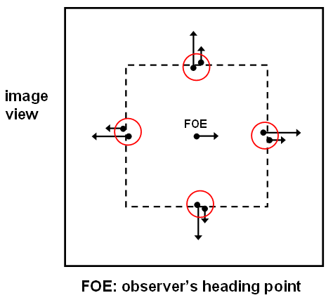
- Turn in a drawing for the following: For each of the four regions circled below, show how this added object motion would alter the difference in velocity measured across the border. Draw the lines that contain the four velocity difference vectors and show roughly where these lines intersect in the image (this is the heading point that would be computed by Longuet-Higgins and Prazdny's algorithm).
- Answer the following question: Can this algorithm compute the correct heading point for these situations where the object undergoes its own motion?
Submission details:
- Hand in a hardcopy of your
ske.mfile - Hand in a hardcopy of your
setupImageVelocities.mfile and - Hand in your written drawings and explanations for problems 2b and 2c.
- Hand in your Discussion Log
- Upload to Canvas the electronic copies of your ske.m and setupImageVelocities.m code files
Home | | Schedule | | Assignments | | Lecture Notes
Constance Royden--croyden@holycross.edu
Computer Science 363--Computational Vision
Last Modified: April 12, 2023
Page Expires: April 12, 2024