CSCI 363 Computational Vision--Spring 2023
Assignments
Home | | Schedule | | Assignments | | Lecture Notes
Assignment 5, Due Thursday, March 30
This assignment contains two programming problems on computing a 2D
velocity field. Images and initial code for the programming problems
are contained in the ~csci363/assignments/assign5 subdirectory
on radius. After copying this folder to your own assign5 directory, set the Current Directory
in MATLAB to this folder.
Problem 1: Motion Correspondence
Problem 1a) Implementing motion correspondence
This problem builds on the previous method that you explored for solving the stereo correspondence problem. In the stereo correspondence problem, every patch of the left image (excluding a border around the image) was compared to a set of horizontally displaced patches in the right image to find the best match and assign a stereo disparity to each location of the left image. In this context, the measure used to assess the quality of the match was the correlation between the pattern of zero-crossings in the left and right image patches. In this problem, the measure you will use to assess the quality of the match is the sum of the absolute differences in intensity between the patch in the first image and the patch in the second image. Instead of maximizing a correlation as in the stereo problem, you will be minimizing the differences in this problem.
In this problem, you will implement a strategy for motion measurement similar to that used in
the previous stereo matching solution. The assign5
folder contains a definition of the stereoMatch function from Assignment 4 that
uses the "sum of absolute differences" measure of similarity instead of the correlation
measure used in assignment 4. Use this function as a starting point to create a function named
motionMatch that computes the motion at each location in a sequence of images.
Your function should have four inputs, similar
to the stereoMatch function, representing the two images in a motion sequence,
an input that indicates the size of the image patches used for matching between the two images
(nsize) and an input range that specifies the range of displacements
of the patches in the horizontal and vertical directions to be considered by the function. For
each patch in the first image (ignoring a border around the image), the function should
find a patch in the second image that is the best match, and record both the
horizontal and vertical displacements between the two patches. These displacements should be
recorded in two separate matrices that are provided as outputs of the function. The
testMatch.m script in the assign5 folder contains code to test your
motionMatch function that reads in two images from the assign5 folder,
shows the images as a movie, and creates and displays the true velocity field for the images.
In comments, there is code to run your motionMatch function on these two images.
Compare your results to the true velocity field.
Question 1b)
In a separate document, answer the following question:
Where do the errors occur in the results, and why
might you expect errors in these regions?
Problem 2: Computing the velocity field
Problem 2a) Computing the velocity field
In this problem, you will write a function named computeVelocity whose input
includes the perpendicular components of motion derived from two images in a motion
sequence, and whose output is a 2D velocity field.
In class, we developed an algorithm to compute 2-D velocity from the perpendicular components
of motion, assuming that velocity is constant over extended regions in the image. Let
(Vx,Vy) denote the 2D velocity,
(pxi,pyi) denote the unit vector in the direction of
the gradient (i.e. perpendicular to an edge) at the ith image location, and
vpi denote the perpendicular component of velocity at this
location. In principle, from measurements of pxi, pyi and
vpi at two locations, we can
compute Vx and Vy by solving the following
two linear equations:
Vx px1 + Vy py1 =
vp1
Vx px2 + Vy py2 =
vp2
In practice, a better estimate of (Vx,Vy) can be obtained
by integrating information from many locations, and finding values for Vx and
Vy that best fit a large number of measurements of the perpendicular
components of motion. Because of error in the image measurements, it is not possible to find values for
Vx and Vy that exactly satisfy a large number of
equations of the form:
Vx pxi + Vy pyi = vpi
Instead, we compute Vx and Vy that minimize the difference
between the left- and right-hand sides of the above equation. In particular, we compute
a velocity (Vx,Vy) that minimizes the following expression:
∑[Vx pxi + Vy pyi -
vpi]2
where ∑ denotes summation over all locations i. To minimize this
expression, we compute the derivative of the above sum with respect to each of the two parameters
Vx and Vy, and set these derivatives to zero. This
analysis yields two linear equations in the two unknowns Vx and Vy:
a1 Vx + b1 Vy = c1
a2 Vx + b2 Vy = c2
where
a1 = ∑pxi2
b1 = a2 = ∑pxipyi
b2 = ∑pyi2
c1 = ∑vpipxi
c2 = ∑vpipyi
The solution to this pair of equations is given as follows:
Vx = (c1b2 -
b1c2)/(a1b2 - a2b1)
Vy = (a1c2 -
a2c1)/(a1b2 - a2b1)
Your computeVelocity function will implement this solution.
The function getMotionComps, which is already defined in the assign5
folder, computes the initial
perpendicular components of motion. This function has three inputs - the first two are
matrices containing the results of convolving two images with a Laplacian-of-Gaussian function.
It is assumed that there are small movements between the original images. The
third input to getMotionComps is a limit on the expected magnitude of the
perpendicular components of motion. This function has three outputs that are matrices containing
values of px, py and
vp. These quantities are computed only at the
locations of zero-crossings of the second input convolution. At locations that do not
correspond to zero-crossings, the value 0 is stored in the output matrices.
Your computeVelocity function should have the following header:
function [vx vy] = computeVelocity (px, py, vp, nsize, step, vlim)
The inputs px, py and vp are the three matrices that are returned by
the getMotionComps function. nsize is a neighborhood size for
integrating the motion components to compute the velocity at a particular location. To reduce the
amount of computation, velocities do not need to be computed at every location. Instead,
velocities should be computed at evenly spaced locations in the horizontal and vertical directions,
with the input step specifying the space between these locations.
Finally, vlim is a limit on the expected horizontal and vertical velocities that should
appear in the results. The two outputs of the computeVelocity function are matrices
of the same size as the input matrices, containing values for
Vx and Vy at the locations where velocity was
computed, and the value 0 elsewhere.
The computeVelocity function should step through the equally spaced image locations,
and at each location (x,y), it should
integrate all of the measurements of px, py and
vp within a square region from
(x-nsize,y-nsize) to (x+nsize,y+nsize) and compute the coefficients
a1, a2, b1, b2, c1 and
c2 (remember to initialize these coefficients to
0 before accummulating
information for each new region). The velocity for the region should then be computed by solving for
Vx and Vy as shown above. If the absolute values of
both Vx and Vy are within the limit vlim,
then Vx and Vy
should be stored at the corresponding locations in the output matrices vx and
vy.
The motionTest.m script file contains two examples for testing your new function. The
first example uses images of a circle translating down and to the right. The second example,
which is initially in comments, uses a collage of four images of Red Sox players from the 2007
World Series team,
where each subimage has a different motion, as shown by the red arrows on the image below:
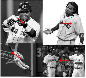
Big Papi is shifting down and to the right, Manny Ramirez is shifting right, Jason Varitek and Mike Lowell are
shifting left, and Coco Crisp is leaping up and to the left after a fly ball. For both examples,
the velocities computed by your computeVelocity function are displayed by
the displayV function in the assign5 folder, which uses the built-in
quiver function to display arrows. Your results for the Red Sox image should roughly
reflect the correct velocities within the four different regions of the image, but there will be
significant errors in some places.
Question 2b) In a separate document, answer the following
question:
Where do most of the errors in the results occur, and why might you expect
errors in these regions?
The results of your implementation will vary, depending on the size of the neighborhood used
to integrate measurements of the perpendicular components of motion. Run your
computeVelocity function with a larger and smaller neighborhood size and describe
the change in results.
Question 2c)
What are possible advantages or disadvantages of using a larger
or smaller neighborhood size for the computation of image velocity?
Problem 3: Project Proposal
First, choose a partner for your project. Include this in your written answers to
Assignment 5 by Thursday, March 30.
Read the
Project description for the project.
Project proposal, due Tuesday, April 11: Write a paragraph
description of your topic and include at least one reference that you will use in your
research of your topic.
Submission details:
- Hand in a hardcopy of your
motionMatch.mcode file - Hand in a hardcopy of your
computeVelocity.mcode file - Hand in your answers to the questions for Problems 1-3.
- Turn in a hardcopy of your project proposal in a separate document by Tuesday, April 11.
- Upload to Canvas an electronic copy of your code files for motionMatch.m and computeVelocity.m
Home | | Schedule | | Assignments | | Lecture Notes
Constance Royden--croyden@holycross.edu
Computer Science 363--Computational Vision
Last Modified: March 22, 2023
Page Expires: March 22, 2024