CSCI 363 Computational Vision--Spring 2023

Assignments

Home | | Schedule | | Assignments | | Lecture Notes

Assignment 4, Due Thurs, March 23

In this assignment, we will work with several different algorithms for computing stereo disparity-- Marr-Poggio, Marr-Poggio-Grimson and a correlation algorithm that you will write yourself. These algorithms make use of constraints for matching features in the left and right images, such as continuity and similarity.

Files needed for this assignment

Problem 1: The Marr-Poggio stereo algorithm

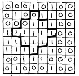
In this problem you will implement the Marr-Poggio stereo algorithm and see how it computes stereo disparity for a random dot stereogram over repeated iterations using the four constraints discussed in class. First, run the script, stereoScript, to create a random dot stereogram of concentric circles at different disparities. The center circle is closest to the observer, and each wider circle is a little further back, so it looks like viewing a wedding cake from above. The stereogram is shown two ways--as a left and right image of random white and black dots, and as a red-green stereo pair (anaglyph). Use the red-green glasses in lab to view the red-green image to see the "cake." You can see how the stereogram is created by viewing the functions, makeCake.m and makeStereogram.m

Now you will complete the function, final_net = coopStereo(left, right, minD, maxD, iters) to implement the Marr-Poggio algorithm. In this function the left and right parameters specify the left and right stereo images. minD and maxD specify the minimum and maximum disparities used in the stereogram and iters is the number of iterations the algorithm should be run. Write your code using the following steps:

• Open the function file, called coopStereo.m
• Create two new 3D arrays (net1 and net2 filled with zeros. The dimensions should have the same x, y dimensions as the input stereogram and the third dimension equal to the disparity range.
• Write a nested for loop to initialize the network, net1, by stepping through all the rows and columns and disparities. The value in net1 should be set to 1 if left(i, j) is equal to right(i, j + disp).

  Leave 2 rows of zeros at the top and the bottom of net1, and dRange columns of zeros on the left and right side of net1

  Note that the second value is the column number, so it indicates horizontal position.

  Also note that when the disparity is the minimum disparity, the index of the third dimension is one, so you will have to take that into account to make sure the correct position in the array is initialized.

• The next set of nested for loops is used to iterate through the algorithm. For each iteration, they loop through all rows, columns and disparities. Your job is to compute the positive and negative support at each position and then test to see if the network should have a 1 or a zero in the next iteration.
• First, compute the positive support by adding together the values in all the neighboring positions at the current disparity. The pattern of neighbors to add in is shown below.

  

• Second compute the negative support by adding together all the other possible matches. These are the places where there is a one at the same (x,y) position and a different disparity: net1(i, j, disp), or at a position along a diagonal through that position: net1(i, j+d-disp, disp).

  Use a for loop to add together all the ones in these positions from disp = 1 to dRange.

  Subtract out two times the value of the current position: net1(i, j, d)

• Test to see if the total support is greater than the threshold and set corresponding net2 value to 1 if the total support is greater than threshold and zero if it is not. Total support is computed as the current value in net1 plus the positive support minus epsilon times the negative support.

When you are done, you can test your algorithm by uncommenting the last two lines of stereoScript.m, and running that script. This will run 5 iterations of your algorithm. You should see the concentric circles emerge.

Hand in: A hard copy of coopStereo.m with your assignment 4 and upload the code file to Canvas.

Problem 2: The Marr-Poggio-Grimson Multi-resolution Stereo Algorithm

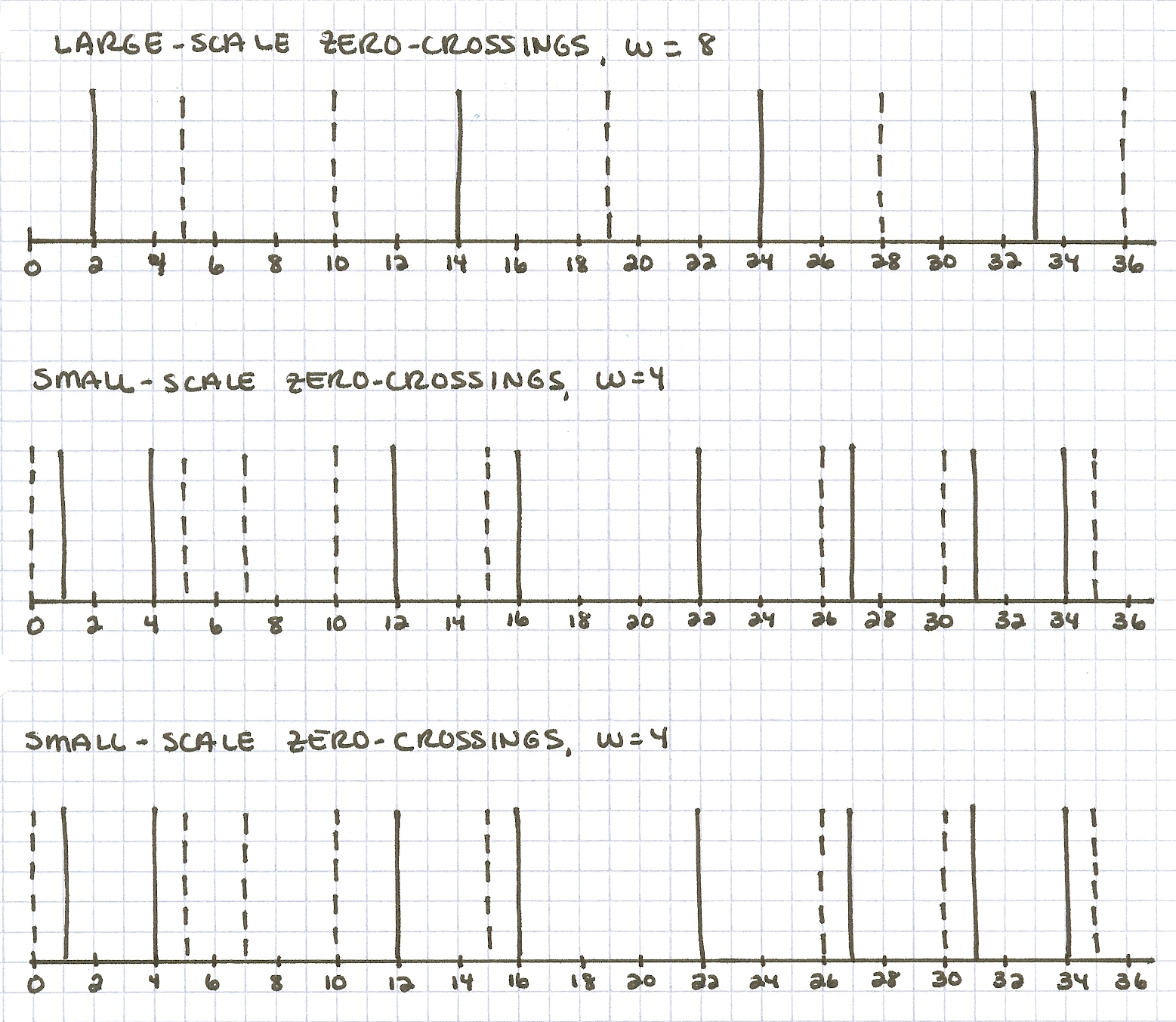
In class, we discussed a simplified version of the MPG multi-resolution stereo algorithm and performed a hand simulation of this algorithm on the board. This problem provides another example for you to hand simulate on your own. The zero-crossing pictures are shown below. The top row shows zero-crossing segments obtained from a Laplacian-of-Gaussian operator whose central positive diameter is w = 8, and the bottom two rows show zero-crossing segments obtained from an operator with w = 4. Assume that the matching tolerance m (the search range) is m = w/2. In the diagram, the solid lines represent zero-crossings obtained from the left image and the dashed lines are zero-crossings from the right image (assume that they are all zero-crossings of the same sign). The axis below the zero-crossings indicates their horizontal position in the image.

Part a: Match the large-scale zero-crossing segments. In your answer, indicate which left-right pairs of zero-crossings are matched and indicate their disparities.

Part b: Match the small-scale zero-crossings, ignoring the previous results from the large-scale matching. In your answer, indicate which left-right pairs of zero-crossings are matched and indicate their disparities. Show your analysis for this case on the bottom row of the figure.

Part c: Match the small-scale zero-crossings again. This time exploit the previous results from the large-scale matching. Show your analysis for this case on the middle row of the figure.

Part d: What are the final disparities computed by the algorithm, based on the matches from Part c? The final disparity is defined as the shift in position between the original location of the left zero-crossings and the location of their matching right zero-crossings.

Part e: One of the constraints that is used in all algorithms for solving the stereo correspondence problem is the continuity constraint. What is the continuity constraint, and how is it incorporated in the simple version of the MPG stereo algorithm that you hand-simulated in this problem?

Problem 3: A Stereo Algorithm Based on Correlation

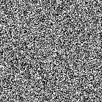
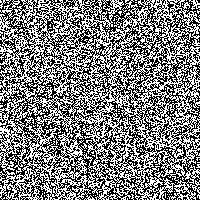
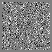
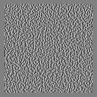
In this problem, you will implement a stereo correspondence algorithm based on a strategy known as correlation. The input for this new algorithm will be the zero-crossings computed by the stereoZeros function given to you. In the figure below, the top left and right pictures show a random-dot stereogram with a central square patch that has a disparity of +2 pixels and a background disparity of +1 pixels. The middle left and right pictures show the zero-crossings obtained from convolving the two images with a Laplacian-of-Gaussian operator of size w = 4. Positive zero-crossings are shown in white and negative zero-crossings in black. Your task is to write a function called stereoMatch that solves the correspondence problem and computes a disparity for each location in the left image. The bottom picture in the figure below shows sample results from an implementation of stereoMatch. The function computed a disparity of +2 for central locations in the image (displayed in white) and a disparity of +1 for the surrounding region (displayed as gray). There is a border around the outside of the image where disparities are not computed (zero values, shown in black).

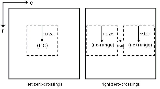
The figure below illustrates the strategy that you should use to solve the stereo correspondence problem. Assume that the left and right input pictures contain the zero-crossings derived from the original left and right stereo images. Suppose we want to compute the disparity at location (r,c) (row r and column c) in the left picture. Consider a square neighborhood that extends nsize pixels in the four directions around location (r,c), as shown in the left picture below. To compute a disparity for this location, your function should search in the right picture for a square patch of the same size that best matches the content of the left patch. To find the most similar patch in the right picture, consider a range of possible horizontal positions of the patch centered on locations (r,c-range) to (r,c+range), as shown in the right picture below. The horizontal position of the most similar patch in the right image, relative to the position of the original patch in the left image, determines the disparity assigned to location (r,c).

For this problem, you will use a measure of similarity between two patches based on correlation. Correlation is a general computational technique that arises in many image processing applications and in the description of models for biological computations. Correlation is similar to convolution. The picture below shows two small image patches labeled I1 and I2 that each contain the three values -1, 0 and +1 (similar to a zero-crossing representation):

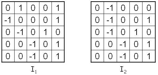
The correlation between the two image patches is defined as:

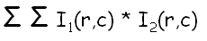
where the summation is performed over the entire 2D region. The values in the two patches are multiplied point-by-point and the products are then summed. For the above images, the pointwise multiplication yields the following intermediate result:

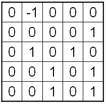
The sum of all of these products is 6. In this simple case where the images contain only -1, 0 and +1, the pointwise product will be 1 at a location where both image patches contain +1 or both image patches contain -1. If the two patches contain opposite values at the same location (i.e. -1 and +1), their product will be -1. If we now think of the +1 and -1 values in the input left and right patterns as representing positive and negative zero-crossings, then this correlation measure effectively adds up the number of locations that contain zero-crossings of the same sign in the two image patches, and subtracts the number of locations that contain zero-crossings of opposite sign in the two patches. Thus, this correlation measure gives a rough indication of how well the zero-crossings match between two image patches. As the similarity of the zero-crossings in the two patches increases, the correlation increases. Therefore a patch in the right pattern that best matches a given patch in the left pattern will have the maximum correlation value.

As stated earlier, your task is to define a function stereoMatch that uses the approach described above to solve the stereo correspondence problem. Your function should have the following header:

function result = stereoMatch (zcleft, zcright, nsize, range)

The correlationScript.m file contains a sequence of statements that create a stereogram (using the chapelLeft.jpg and chapelRight.jpg images), use the conv2D function to convolve the left and right images with a Laplacian-of-Gaussian operator (using a value of w = 4), compute the zero-crossings with the stereoZeros function, and runs the stereoMatch function to compute disparities, and display the results. An operator size of w = 4, disparity range of 6 and neighborhood size of 10 is used to produce good results.

Run the correlationScript to test your algorithm.

This stereo pair is constructed from a real image (you can see it by typing chapel = imread('chapelLeft.jpg') and then using imtool(chapel)) and a disparity pattern that conveys a secret message that you can view. If you don't see a readable message, you have not correctly written your stereoMatch function.

Problem 4: The Correlation-Based Stereo Algorithm

We discussed four constraints that most stereo correspondence algorithms incorporate: uniqueness, similarity, continuity and the epipolar constraint. Explain how the correspondence-based strategy that you implemented in Problem 3 uses each of these four constraints.

Submission details:

• Hand in a hardcopy of your coopStereo.m and stereoMatch.m code files
• Hand in a hardcopy of your answers to the questions for Problems 1-4.
• Hand in your discussion log
• Upload to Canvas your code files for coopStereo.m and stereoMatch.m

Home | | Schedule | | Assignments | | Lecture Notes

Constance Royden--croyden@holycross.edu
Computer Science 363--Computational Vision
Last Modified: March 13, 2023
Page Expires: March 13, 2024